Overview
TeX is a low-level typesetting system created by Donald Knuth in 1978 at Stanford University. The name was original composed of the Greek letters tau, epsilon, and chi (which looks like the Latin letter X). That is why TeX is pronounced “tech” and not “tex”.
LaTeX is a high-level typesetting system built on TeX by defining a set of custom TeX commands. The initial version was created by Leslie Lamport in 1984. The latest version was implemented by a group led by Frank Mittelbach. LaTeX is widely used in academia for publication of technical articles, papers, and books. It is typically used to produce PDF files, but can also produce DVI (device independent), EPUB, HTML, Markdown, MathML, plain text, Postscript, SVG, and Word files.
The additional programs BibTeX and MakeIndex are used to generate
bibliography and index pages.
LaTeX is pronounced “Lah-tech” or “Lay-tech”. It is not pronounced the same as “latex”, the substance that comes from trees and plants which is used to produce rubber.
Both TeX and LaTeX are markup languages that are
used in text files with a .tex file extension.
Other commonly used markup languages include HTML, Markdown, SVG, and XML.
Pros and Cons
Some pros of using LaTeX include:
- provides high-quality typesetting for professional looking PDF documents, especially those that contain mathematical equations
- allows authors to focus on content before formatting while maintaining consistent formatting and automatic numbering of pages, chapters, sections, figures, and tables (uses a separate “counter” for each kind of content)
- supports extensive customization through thousands of packages and templates for various document types
- supports generating a table of contents, list of figures (images), list of tables, footnotes, bibliography (with references), and an index
- scales to support large projects like books and theses by allowing documents to be split into multiple files
- supports defining parameterized macros that reduce duplicated code
- cross-platform, running in Windows, macOS, and Linux
- free and open source
- being text-based enables easy viewing of diffs in version control systems
Some cons of using LaTeX include:
- steep learning curve for its markup syntax
- customizing layouts and formatting can be time-consuming
- markup syntax must be compiled in order to view what will be rendered in the target output (often a PDF)
- error messages can by cryptic
- creating tables and managing placement of images can be more cumbersome compared to many word processing applications
- collaboration requires all contributors to have knowledge of LaTeX
Installing
Generating PDF documents from LaTeX documents requires a distribution and an editor.
The distribution provides executables that must be found
in a directory listed in your PATH environment variable.
The TeX Live
distribution is recommended.
Installing in macOS
The macOS version of TeX Live is named mactex.
One way to install mactex is to install Homebrew
and then enter brew install mactex.
This installs the following shell commands:
| Command | Description |
|---|---|
pdflatex | compiles .tex files into PDF format |
xelatex | like pdflatex, but supports TrueType font, OpenType fonts, and Unicode |
lualatex | like xelatex, but supports Lua scripting |
latex | compiles .tex files into DVI (older format) |
dvips | converts DVI files to PostScript |
dvipdfmx | converts DVI files to PDF |
bibtex | processes .bib files for bibliography references |
biber | more powerful bibliography processor (alternative to bibtex) |
makeindex | generates an index for documents |
tlmgr | TeX Live package manager (for installing/updating LaTeX packages) |
kpsewhich | searches for installed TeX files |
texhash | updates TeX’s file database after installing packages |
latexmk | automates LaTeX compilation (runs multiple passes as needed) |
Installing in Windows
There preferred LaTeX distribution for windows is MiKTeX.
Installing in Linux
Many Linux distributions come with the commands needed to process LaTeX documents already installed.
Command-line Processing
To generate a .pdf file from a .tex file in a terminal window,
run one of the following commands:
pdflatex {name}.tex
xelatex {name}.tex
lualatex {name}.tex
It is sometimes necessary to run these commands multiple times in order to get the desired result. The first run gathers information about the document, such a page numbers where figures and tables appear, and writes it to special files (described later). These files are used to produce the final output, but on the first run the output is be produced using the previous versions of these special files.
Everything these commands write to the terminal
is also written to the file {name}.log.
However, when using the VS Code extension “LaTeX Workshop”,
it seems to delete the log file.
Open the generated PDF document with the following command:
open {name}.pdf
TeX editors will handle both of these steps for you.
Error Handling
Common errors encountered when processing .tex files include:
- misspelled command, environment, or declaration name
- mismatched braces or other delimiters
- command missing a required argument
- attempting to print a special character without escaping it
- use of syntax that is only valid in math mode outside of math mode
If an error is encountered, an error message will appear in the terminal.
The message will begin with ! and be followed by
“LaTeX Error:” if it was detected by LaTex rather than by TeX.
The next line will include the line number where the error occurred.
The final line will only contain ?.
To continue processing, press the return key. This allows viewing multiple errors that can all be fixed before the next run.
To stop processing, type x and press the return key (or press ctrl-d).
If the final line only contains *,
it is likely that the \end{document} command was not found.
Press ctrl-d to exit and add the missing command.
Editors
Recommended LaTeX editors include TeXmaker, VS Code, and Overleaf.
TeXmaker
TeXmaker is a free, cross-platform LaTeX editor. Download the installer, run it, and drag the app icon to the Applications directory. Double-click the app to run it. It will likely show an error dialog that says “texmaker.app is damaged and can’t be opened”, but it is not damaged. To fix this, open a terminal window and enter the following command:
sudo xattr -dr com.apple.quarantine /Applications/texmaker.app
VS Code
VS Code can be used to edit .tex files.
Install the extension “LaTeX Workshop” from James Yu.
This automatically generates a PDF
every time changes to a .tex file are saved
and the PDF can be viewed inside VS Code.
When changes to a .tex file are saved, the “LaTeX Workshop” extension
“Build LaTeX project” command will automatically run.
There is also a right-pointing green triangle in the upper-right
that can be clicked to run that same command.
To view the PDF, click the preview button in the upper-right that looks like a two-page document with a small magnifier glass on top of it.
To jump from a \ref{label} command in the .tex file to the
corresponding location in the generated PDF displayed in the preview,
hover over the label text and click “View on pdf”.
To jump from the content under the cursor in the .tex file to the
corresponding location in the generated PDF displayed in the preview,
press cmd-option-j.
To jump from a location in the PDF preview to the
corresponding location in the .tex file, command-click it.
LaTeX Workshop defines snippets to simplify entering some commands.
For example, BIT expands to the following:
\begin{itemize}
  \item
\end{itemize}
The BEN snippet is similar, but uses enumerate.
The BFI snippet expands to the set commands typically used to create a figure.
The BTA snippet expands to the set commands typically used to create a table.
For more snippets, see Snippets and shortcuts.
To see a preview of a mathematical expression rendered in a popup,
hover over the opening $, the opening $$,
or the word “align” in \begin{align}.
By default this extension uses the pdflatex command
to generate PDF files. To change this to use xelatex,
which is required for some functionality:
-
Select “Preferences: Open User Settings (JSON)” from the command palette.
-
Search for “pdflatex”.
-
Copy the object containing that immediately after it.
-
In the copied object, change the values of “name” and “command” from “pdflatex” to “xelatex”.
-
Add the following at the end of the
settings.jsonfile before the closing curly brace:"latex-workshop.latex.recipes": [ { "name": "xelatex", "tools": ["xelatex"] } ], "latex-workshop.latex.recipe.default": "xelatex" -
Open
settings.jsonand modify “latex-workshop.latex.tools”.Add
"-shell-escape",to the “args” arrays for the following commands: latexmk, lualatexmk, xelatexmk, pdflatex, and xelatex.
VS Code can format LaTeX documents, but it the “LaTeX Workshop” extension
does not include a formatter.
latexindent.pl is a Perl script
that formats .tex files and can be used from VS Code.
The “getting started” section of its GitHub README page
explains how to install it for various operating systems.
In macOS, enter brew install latexindent from a terminal window.
To configure they LaTeX Workshop extension to use latexindent,
open Settings, select Extensions…LaTeX.
For “Latex-workshop › Formatting: Latex”, select “latexindent”.
For “Latex-workshop › Formatting › Latexindent: Path”,
if the command latexindent is in your PATH,
this can be set to only latexindent.
To format the .tex file currently begin edited,
right-click anywhere in the document and select “Format Document”,
or open the Command Palette and select “Format Document”.
In order to get latexindent to work, I had to enter the following commands
in a terminal to install additional Perl modules:
cpan YAML::Tiny
cpan File::HomeDir
Overleaf
Overleaf is a web-based editor that doesn’t require installing any software. It requires creating an account. There are free and paid accounts.
Paid accounts have the following features that are not present in free accounts:
- collaborating on documents with multiple editors
- marked issues as resolved
- accept or reject suggested changes
- compiling large documents will not timeout
- document history is maintained
- advanced search
- symbol palette for inserting math symbols with a click
- integrations with version control systems
- technical support
Paid accounts are $199 (10 collaborators per project) or $399 (unlimited collaborators per project) per year.
Syntax
LaTeX documents consist of a sequence of commands and content. Most commands begin with a backslash. Some commands have a second form whose name ends with as asterisk that behave somewhat differently than their non-asterisk form.
LaTeX commands begin with a backslash followed by a name. Some commands have optional and/or required parameters. Optional arguments appear in square brackets separated by commas. Required arguments each appear in their own pair of curly braces.
Optional arguments are positional. If a command accepts two optional arguments and only one is supplied, it is used as the first and the second uses its default value.
The most basic LaTeX document contains the following:
\documentclass{article}

\begin{document}
Hello
\end{document}
All commands begin with a backslash and a name. Command names are case-sensitive and consist of letters, not numbers or other special characters.
Some commands are followed by required arguments where each is contained in its own pair of curly braces.
Some commands take optional arguments where each is contained in its own pair of square brackets. But sometimes all the optional arguments appear in a comma-separated list inside a single pair of square brackets. Usually the optional arguments appear before the required arguments, but sometimes they appear after them.
Many commands support a “star variant” that affects its behavior.
For example, \chapter{some name} starts a new, numbered chapter
and \chapter*{some name} starts a new, unnumbered chapter.
The commands before \begin{document} are referred to as the preamble
which must begin with \documentclass{some-class}.
These commands:
- describe the class of document being created
- optionally import packages which provide support for additional commands
- optionally configure document-wide formatting
The entire content of a document must be surrounded by
\begin{document} and \end{document}.
Declarations
A “declaration” changes the effect of subsequent commands
or the meaning of arguments to subsequent commands.
The scope of the effect is from the declaration to
the next closing curly brace (}) or end of an an environment (\end{name}).
There is a set of special declarations
whose scope extends to the end of the document.
Examples include \pagenumbering and \pagecolor.
For example, the following declaration causes the text inside the curly braces to be huge:
{\Huge Shout it from the rooftops!}
Environments
An “environment” can provide content to be rendered at its beginning and end, and can specify the default formatting of its content.
The \begin{name} command starts a usage of the named environment.
It must be paired with a corresponding \end{name} command.
Some environments take additional arguments
that are specified on the \begin command.
Some environments have a second form whose name ends with as asterisk
that behave somewhat differently than their non-asterisk form.
The following example uses the center environment
which centers each line of text inside it.
The \\ command inserts a newline character.
For more on inserting space, see the “Space” section below.
\begin{center}
  one \\
  two \\
  three \\
\end{center}
Custom environments are defined with the \newenvironment command.
To redefine an existing environment, use the \renewenvironment command.
Environments are typically defined in the preamble.
The following contrived example defines a custom environment
that inserts common starting and ending text of a fairy tale.
The arguments to the \newenvironment command are
the environment name, the beginning text, and the ending text.
\newenvironment{fairytale}
  {Once upon a time,}
  {And they all lived happily ever after.}
The following is an example of using the fairytale environment:
\begin{fairytale}
in a kingdom nestled beside a sparkling sea,
lived a young princess named Aurora.
Her days were filled with laughter and the gentle rhythm of the waves,
until a mischievous sea sprite stole her favorite seashell,
a gift from her grandmother.
\end{fairytale}
The following version of the fairytale environment adds an optional parameter to specify the text color. The parts of the definition, in order are:
- The environment name in curly braces.
- The number of parameters in square brackets.
- The default values for the parameters, each in their own pair of square brackets. Parameters that are not given a default value are required parameters.
- The begin content in curly braces.
- The end content in curly braces.
The parameters can only be used in the begin content.
They are referred to with #1, #2, and so on.
\newenvironment{fairytale}[1][blue]
  {\color{#1}Once upon a time,}
  {And they all lived happily ever after.}
Using declarations instead of commands is especially useful in environment definitions because an environment cannot use a command to wrap around the supplied content. Instead, they can use declarations to change styling for all the text that follows, up to the end of the environment.
The following is an example of using the new version of fairytale environment and specifying green as the text color:
\begin{fairytale}[green]
  in a kingdom nestled beside a sparkling sea, ...
\end{fairytale}
Command Groups
A command group is defined by a pair of curly braces and limits the scope of a command so it only affects the content inside the group. For example, the following causes all the text rendered inside the group to in a huge font.
{\huge
  ...
}
Special Characters
There are ten special characters in LaTeX that require special handling to render as the literal character. The following characters must be escaped with a backslash: $ & # % _ { }.
To render a backslash, use the \textbackslash command.
To render a caret, use the \textasciicircum command.
To render a tilde, use the \textasciitilde command.
To render text in double curly quotes,
begin with two backticks and end with two single quotes.
For example, ``quoted text''.
To render text in single curly quotes,
begin with one backtick and end with one single quote.
For example, `quoted text'.
There are three sizes of dashes:
- intra-word with
- - number ranges with
-- - punctuation with
---
To print accented characters and symbols that appear in non-English text, see LaTeX/Special Characters.
Document Classes
Document classes change the default formatting by redefining environments and commands. They can also define new environments and commands.
Document classes that can be specified in \documentclass[options]{some-class} include:
articlesupports an abstract, sections, and subsections, but not chaptersbeamerfor slide presentationsbooksupports a title page, table of contents, chapters (starting on odd-numbered pages), and bibliographyexamfor lists of questionsleafletlettermemoirbased on thebookclassminimalonly sets page size and a base font (mostly for debugging)paperprocfor proceedings; based on thearticleclassreportfor documents with chaptersslidesfor slide presentations, butbeameris preferred
Options that can be specified in this command include:
-
draftorfinal(default)When in draft mode:
- Lines in boxes that are too long to fit within the page margins are highlighted with black bars in the margin.
- All figures are replaced with empty boxes of the same size that contain image file paths. These can help with diagnosing layout issues.
-
flegnto left-align equations rather than center them -
landscapeto use landscape orientation rather than portraitThis requires using
xelatexorlualatexinstead ofpdflatex. -
legnoto place equation numbers on their left side rather than right side -
openbibto use the “open” bibliography format -
openany(default) oropenrightto begin chapters on right-hand pages whentwosideis used -
titlepage/notitlepageto specify whether there should be a title pageThis seems to have no effect. A title page is generate if and only if the
\maketitlecommand is used. -
onecolumn(default) ortwocolumnto use 2-column pages throughout the entire documentThis requires using
xelatexorlualatexinstead ofpdflatex. -
oneside(default) ortwosideto print on both sides of paper -
a font size which can be one of the following:
10pt(default),11pt, or12pt -
a paper size that can be one of the following:
a4paper: 210 x 297 mm; approx. 8.25” x 11.75”a5paper: 148 x 210 mm; approx. 5.8” x 8.3”b5paper: 176 x 250 mm; approx. 6.9” x 9.8”executivepaper: 7.25” x 10.5”legalpaper: 8.5” x 14”letterpaper: 8.5” x 11”
See the video tutorial at https://www.youtube.com/watch?v=ydOTMQC7np0!
Packages
Packages can add support for additional commands. They can also modify default settings that affect how documents are rendered.
Documentation on all LaTeX packages can be found at Comprehensive TEX Archive Network (CTAN).
To open documentation for a given package from the command line,
enter texdoc {package-name}.
The documentation will open in your default web browser.
To import a package, use the \usepackage command in the preamble.
This can take a set of optional arguments in square brackets.
It also takes a comma-separated list of package names to use in curly braces.
For example:
\usepackage{amsfonts, amsmath, amssymb, amsthm}
\usepackage{float, graphicx}
\usepackage{hyperref}
Popular Packages
In packages whose names begin with “ams”, that stands for American Mathematical Society.
| Package | Description |
|---|---|
| amsfonts | adds fonts for use in mathematics |
| amsmath | adds commands for rendering mathematical formulas |
| amssymb | adds commands for additional mathematical symbols |
| blindtext | generates random text for testing layouts |
| comment | adds support for multi-line comments |
| fancyhdr | adds commands to configure page headers and footers |
| float | improves ability to control placement of objects like figures and tables |
| geometry | adjusts page margins, page size, and layout |
| graphicx | builds on the graphic package to enhance support for graphics |
| hyperref | adds commands to create clickable hyperlinks |
| inputenc | adds support for various input encodings like utf8 |
| lipsum | generates Lorem Ipsum text for testing layouts |
| listings | adds commands to typeset programming language source code |
| minted | formats and highlights programming language source code |
| xcolor | adds commands to change the color of text |
Abstract
To add an abstract section to an article:
\begin{abstract}
  This is the abstract.
  \newpage
\end{abstract}
Sections
Documents can have up to seven levels of sections,
but not all of them are supported for every document class.
For example, the \chapter command can be used
in the document classes book and report,
but not in the document class article.
The following example shows how to specify all seven levels. They must appear in this order without skipping levels.
\part{First Part}
This is a paragraph in a part.

\chapter{First Chapter} % not supported by the article document class
The content of a chapter appears here.

\section{First Section}
The content of a section appears here.

\subsection{First subsection}
The content of a subsection appears here.

\subsubsection{First Subsubsection}
The content of a subsubsection appears here.

\paragraph{First Paragraph}
Any number of paragraphs can appear here.

\subparagraph{First Subparagraph}
Any number of paragraphs can appear here.
Unless the document is a book, the most common kinds of sections to use
include \section, \subsection, and \subsubsection.
The styling of section titles, including whether numbering appears, is determined by the document class.
Parts, chapters, sections, and subsections are automatically assigned increasing numbers starting from 1. Subsubsections, paragraphs, and subparagraphs are not assigned numbers.
To suppress numbering of a chapter, section, or subsection, include an asterisk at the end of its command name. This is commonly do for sections like a preface. When a table of contents is being generated, unnumbered chapters and section not appear in the table of contents.
The fncychap package makes chapter titles fancier.
The options include Bjarne, Bjornstrup, Conny, Glenn, Lenny, Rejne, and Sonny.
For example:

\usepackage[Bjornstrup]{fncychap}
\usepackage[Glenn]{fncychap}
Unicode Characters
To enable the use of Unicode characters, add the following in the preamble:
\usepackage[utf8]{inputenc}
This may only be needed when using pdflatex
and not when using xelatex or lualatex.
In addition, ensure that the selected font contains all the Unicode characters you wish to use. For example, the default font likely does not contain the Unicode wastebasket character.
Portrait vs. Landscape
By default all pages will be in portrait mode.
To cause all pages to use landscape mode, use the geometry package.
For example:
\documentclass[landscape]{some-class}
OR
\usepackage[letterpaper, landscape]{geometry}
The geometry package can also adjust the page margins.
For example:
\usepackage[margin=1in]{geometry}
OR
\usepackage[
  top=1in, bottom=0.5in, left=0.75in, right=0.75in,
  paperwidth=11in, paperheight=8.5in % landscape
]{geometry}
TODO: Cover configuration to printing 2-sided where the left and right margins alternate.
To cause a specific page to use landscape mode, use the lscape package. For example:
\usepackage{lscape}
...
\begin{document}
...
\begin{landscape}
...
\end{landscape}
...
\end{document}
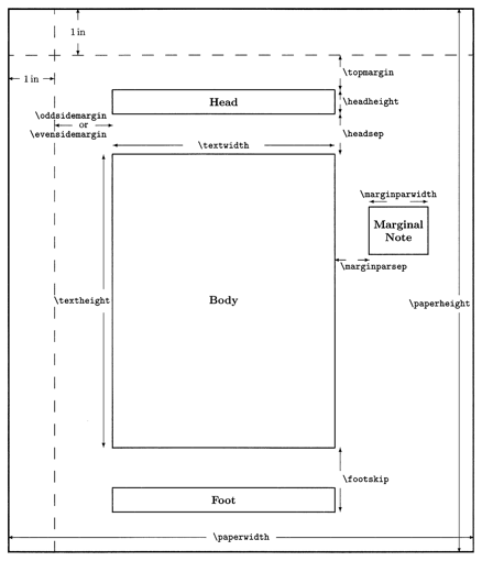
Page Styles
The following diagram shows the commands that can be used to change the layout of pages, including the margins, the sizes of the areas, and the space between the areas.
Page Numbers
Many document classes such as article, book, and report
include page numbers by default.
To suppress the page numbers,
add one of the following commands in the preamble:
\pagestyle{empty}

\pagenumbering{gobble}
The \pagenumbering command can also specify the following values
to use a particular kind of page numbering:
arabic: 1, 2, 3, …alph: a, b, c, …Alph: A, B, C, …roman: i, ii, iii, …Roman: I, II, III, …
Each chapter or section can change the page numbering style and restart page numbering from one. In the following example:
- The title page and table of contents do not have page numbers.
- The pages starting from the preface to before the first chapter use lowercase Roman numerals.
- The remaining pages use Arabic numbers.
The preface chapter is defined with the \chapter* below
to avoid numbering it and cause the first chapter defined with
the \chapter command be considered the first chapter.
\begin{document}
\pagestyle{empty} % removes header and footer from all pages

\maketitle

\tableofcontents
\thispagestyle{empty} % only affects the current page

\chapter*{Preface}
\pagenumbering{roman}
\setcounter{page}{1}
\addcontentsline{toc}{chapter}{Preface}
Preface content goes here.

\lstlistoflistings % requires the listings package
\addcontentsline{toc}{chapter}{\lstlistlistingname}

\listoffigures

\listoftables

\pagestyle{fancy}
\chapter{Jumping In}
\pagenumbering{arabic}

...

\section{Choosing a Tech Stack}
Section content goes here.

\section{Using htmx Attributes}
Section content goes here.

\section{Creating Your First Project}
Chapter content goes here.

\chapter{All About Tables}
Chapter content goes here.

\printindex

\end{document}
Unfortunately, changing the page numbering style breaks
the index generated by the imakeidx and makeidx packages.
See the “Index” section.
Page Headers and Footers
The fancyhdr package enables customizing the content
of the page headers and footers.
The header and footer can render text in three areas,
left, center, and right.
These can differ based on whether the page is even or odd.
For example, the following somewhat matches
the convention followed by Pragmatic Bookshelf books.
All of this must appear in the preamble.
\usepackage{fancyhdr}
\pagestyle{fancy}

% \fancyhead{} % clears default header
% \fancyfoot{} % clears default footer (no more page numbers)
\fancyhf{} % clears both the default header and footer

% Redefine \chaptermark to omit chapter number.
%\renewcommand{\chaptermark}[1]{\markboth{#1}{}}

% Redefine \sectionmark to omit section number.
\renewcommand{\sectionmark}[1]{\markright{#1}}

% L = left, C = center, R = right, E = even pages, O = odd pages
% \leftmark renders the current chapter number and title.
% \rightmark renders the current section number and title.

% This renders the chapter title on the left side of all even pages.
\fancyhead[LE]{\nouppercase{\leftmark}} % chapter title

% This renders the section title on the right side of all odd pages.
\fancyhead[RO]{\rightmark} % section title

% This renders the page number on the left side of even pages
% and the right side of odd pages.
\fancyfoot[LE,RO]{\thepage}
Comments
Single-line comments begin with % and extend to the end of the line.
For example:
% This is a single-line comment.
The “comment” package adds support for multi-line comments. For example:
\usepackage{comment}
...
\begin{comment}
This is a
multi-line comment.
\end{comment}
An alternative way to remind yourself to make a change to the document
is to use the \typeout command which writes its argument to stdout
where the command to process the document is running.
For example:
\typeout{Add more dogs in this table.}
Basic Formatting
The following commands change the formatting of text in their argument.
\textbf{This is bold.}
\textmd{This is medium.} % typically the default
\textit{This is italic.}
\textsc{This is small caps.}
\textsl{This is slanted.} % similar to italic
\textup{This is upright.} % the default

\underline{This is underlined.} % line below
\emph{This can be underlined or italic.}

\textbf{\textit{\underline{bold, italic, and underline}}}

\textrm{This uses a Roman font.}
\textsf{This uses a sans serif font.}
\texttt{This uses a typewriter font.} % monospace
An alternative to using these commands is to use a declaration.
A declaration stays in effect until the next
right curly brace or \end command is reached.
For example, the declaration \em corresponds to the \emph command.
Every declaration has a corresponding environment with the same name.
For example, {\em ... } can be replaced by \begin{em} ... \end{em}
which feels more explicit.
Macros
Macros make it unnecessary to repeat commonly used content and sequences of commands. They can significantly reduce the amount of markup required in documents.
Typically all macros are defined in the preamble. Macro definitions must appear before they are used.
The \def command is a TeX primitive that defines a new command
that can optionally have required parameters.
The \newcommand command uses \def.
Unlike \def, it checks whether the command being defined already exists.
It also adds support for optional arguments.
Here’s an example of defining a macro using \def
which just inserts some static text.
\def\email{someone@gmail.com}
To use this, add \email everywhere that content should be inserted.
Here’s an example of defining a macro using \newcommand.
The command being defined is \image and it takes three arguments.
The arguments are inserted where #1, #2, and #3 appear.
\newcommand{\image}[3]{
  \begin{figure}[H] % see "here" in Figures section
    \centering
    \includegraphics[width=#2]{#1}
    \caption{#3} % see "\caption" in Figures section
  \end{figure}
}
To use this, add \image followed by the three arguments,
each in their own pair of curly braces.
For example:
\image{smalltalk-balloon}{3in}{Smalltalk Programming}
This greatly simplies adding images in a document as long as all should be centered and have a caption.
For custom commands that must be evaluated in math mode,
regardless of whether they are applied in math mode,
wrap the command contents in the \ensuremath command.
Defining a command that already exists with \newcommand
results in an error.
To redefine an existing command, use the \renewcommand instead.
To define a command only if it doesn’t already exist,
use the \providecommand command instead.
Conditional Logic and Iteration
The ifthen package adds commands that support
conditional logic (\ifthenelse command) and iteration (\whiledo command)
for choosing the text to render.
These can be used anywhere in a document, including in macros.
See Master Loops & Conditionals in LaTeX: Beginner.
Fonts
Font Family
To change the font family for a section of the content, surround it with:
textrm{ ... }for a serif font (Roman)textsf{ ... }for a sans serif fonttexttt{ ... }for a typewriter (monospace) font
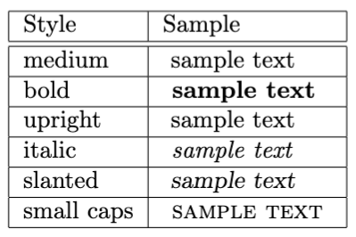
Font Style
To change the font style for a section of content, surround with commands shown in the following table. The style “upright” seems to be same as “medium”.
Font Size
To change the default font size for the entire document,
modify the \documentclass command as follows:
\documentclass[12pt]{book}
For some reason the only font sizes that can be specified here
are 10pt, 11pt, and 12pt.
To change the font size of a section of the content,
surround it with {\size ... } where size is one of
tiny, scriptsize, footnotesize, small, normalsize,
large, Large, LARGE, huge, or Huge.
The font size used by each of these depends on the default font size.
These commands cannot be used in math mode.
For example:
{\huge
some content
}
A specific font size is specified with \fontsize{size}{baselineskip}
where size the font point size and baselineskip is
the distance between the baselines of each line of text.
The baselineskip value will be ignored unless each paragraph,
including the last, is followed by a blank line.
For example:
{\fontsize{18pt}{24pt}\selectfont
Come and listen to a story about a man named Jed
A poor mountaineer, barely kept his family fed,
Then one day he was shootin at some food
And up through the ground came a bubblin crude.

Oil that is, black gold, Texas tea.

Well the first thing you know ol Jed's a millionaire,
Kinfolk said "Jed move away from there"
Said "Californy is the place you ought to be"
So they loaded up the truck and moved to Beverly.

}
TrueType and OpenType Fonts
The shell command pdflatex only supports using Type1 and bitmap fonts,
not TrueType or OpenType fonts.
The shell cvommands xelatex and lualatex
both support TrueType and OpenType fonts.
To use those kinds of fonts:
-
Use the
fontspecpackage.\usepackage{fontspec} -
Specify the font to use with a relative file path or the name of an installed font.
\setmainfont{Pangolin-Regular.ttf} % relative file path. \setmainfont{Apple Chancery} % installed font name -
Use
xelatexorlualatexinstead ofpdflatexto generate a PDF document.xelatex some-name.tex
Colors
The color package provides basic support the changing text color.
\usepackage{color}
...
% Change text color within a group
{\color{red} This text will be red.}
% Or with a command
\textcolor{blue}{This text will be blue.}
The xcolor package provides more features and color models
than the color package and is recommended.
The following color models are supported: cmy, cmyk, gray, Gray, HSB, hsb, HTML, natural, rgb, and RGB.
The following commands provide several examples of rendering text in a specific color:
\usepackage[dvipsnames]{xcolor} % dvipsnames gives 68 more predefined colors.
...

% Using a color name from a small set.
\textcolor{red}{This is red.}

% rgb color
\textcolor[rgb]{0.5, 0.1, 0.9}{Custom purple text}

% HTML color
\textcolor[HTML]{00FF00}{Hex green}

% cmyk color
\textcolor[cmyk]{1,0,0,0}{CMYK cyan}

% Defining a name for a custom color and using it.
\definecolor{darkblue}{RGB}{0,0,102}
\textcolor{darkblue}{This is dark blue text}

% Defining a command for a custom color and using it.
\newcommand{\important}[1]{\textcolor{red}{#1}} % in preamble section
This is a \important{serious issue!}.

% Setting the default color for all the text remaining in a block.
\begin{center}
  \color{purple}
  one \\
  two \\
  three \\
\end{center}

% Rendering text in a box with a colored background.
\colorbox{yellow}{Text with yellow background}

% Rendering text in a box with a colored border and a colored background.
\fcolorbox{red}{lightgray}
  {Red-bordered box with gray background and black text}
To change the background color of pages, use the \pagecolor command.
This stays in effect until another \pagecolor command changes the color.
A limited set of color names are recognized, including
black, white, red, yellow, green, cyan, blue, and magenta.
Use the \definecolor command to define more color names.
For example:
\definecolor{lightgray}{gray}{0.8} % uses gray color model
\definecolor{lightmagenta}{rgb}{1, 0, 1} % uses RGB color model
\pagecolor{lightgray}

% Add page content here.

\newpage
\pagecolor{white} % resets background color for subsequent pages
For more colors, see LaTeX Color.
Lengths
Many commands take a length argument that must include a unit. The supported units are:
cm- centimetersem- width of an uppercase M in the current font (for horizontal lengths)ex- height of a lowercase x in the current font (for vertical lengths)in- inchesmm- millimeterspt- points\baselineskip- line height (distance from the bottom of one line to the bottom of another in the same paragraph)\parindent- width of paragraph indentation\textheight- height of page text area\textwidth- width of page text area
Paragraphs
Paragraphs are separated by blank lines which introduce “hard returns”.
A period is treated as the end of a sentence
unless it is preceded by an uppercase letter.
If a period that does not end a sentence appears in one
(such as etc.), follow the period with a backslash and a space.
By default, the first line in each paragraph
except the first in a chapter or section will be indented.
And there will be no extra space separating the pargraphs,
despite having a blank line between them in the .tex file.
To opt for not indenting the first line of each paragraph and
instead add vertical space between them, add \usepackage(parskip).
To customize the first line indentation:
\setlength{\parindent}{1em}
To customize the vertical space between paragraphs:
\setlength{\parskip}{1em}
To insert random text for testing layouts, add the following in the preamble.
% This causes the \blindtext command to render English text
% instead of the default Latin Lorem ipsum text.
% Omit this line to get Lorem ipsum text.
\usepackage[english]{babel}

% The `random` option causes random text to be generated.
% The `math` option is like the `random` option,
% but also includes random math in the generated text.
% These options only works when the "english" option is specified above.
\usepackage[math]{blindtext}
In the document content, add \blindtext
to insert a single paragraph of random text or
\blindtext[n] to insert n paragraphs of random text.
There are special environments for certain kinds of text.
Poems, haikus, and song verses should appear in a verse environment.
For example:
%\begin{verse}
Out of memory.\\
We wish to hold the whole sky,\\
but we never will.
%\end{verse}
Margin Notes
To place a note in the right margin,
use the \marginpar command immediately after the content
for the line where it should begin.
While there is no limit on the amount of text in the note,
it will not wrap onto another page.
For example:
\marginpar{
  This is a margin note.
}
Space
The LaTeX compiler typically removes extra spaces as it sees fit. A sequence of space characters such as a spaces, tabs, and linefeeds are treated the same as a single space character.
Horizontal Space
There are many ways to insert different amounts of horizontal space. The following options are ordered from least to most space and are depicted in the image that follows. Note the differences in the amount of space between the words “space” and “with”.
\,inserts a thin space\:inserts a medium space\;inserts a thick space\followed by a space inserts an interword space (normal size space)~inserts a normal size space and prevents the next word from appearing on a different line than the previous word (ex.Mr.~Mark~Volkmann)\quadinserts space that is the width of a capital M in the current font (seemining with a thin space on both sides)\qquadinserts double the space inserted by\quad
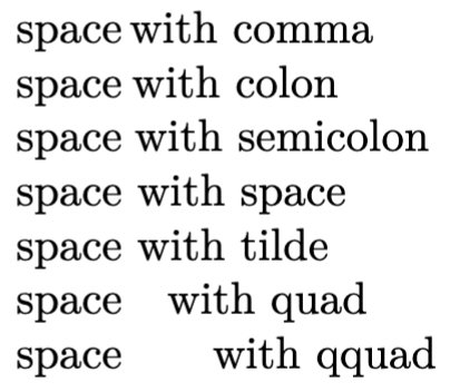
The image above was created with the following markup:
\noindent
space\,with comma\\
space\:with colon\\
space\;with semicolon\\
space\ with space\\
space~with tilde\\
space\quad with quad\\
space\qquad with qquad
To push a single line to the right side of the page,
insert the command \hfill at the begining of the line.
To split the content of a single line so the beginning is at
the left side of the page and the end is at the right side,
insert the command \hfill in the middle of the line.
To insert horizontal space in a line, insert the command \hspace{amount}
where amount is a length value like 1cm.
This is treated like an invisible word of the given length
with a single space on each side that
separates it from the previous and next words.
If the \hspace command ends up at the beginning or ending of a line,
it is removed. Use \*hspace instead to avoid this.
Vertical Space
There are many ways to insert different amounts of vertical space.
By default there is no vertical space betweeen paragraphs
and the first line of each paragraph in each section,
except the first, is indented.
The parskip package can change this.
For example, the following adds vertical space of 14pt between each paragraph
and 20pt of indentation for the first line of each paragraph in each section,
except the first.
\usepackage[skip=14pt, indent=20pt]{parskip}
To add a single newline after a line, add \\ at its end,
which introduces a “soft return”.
To add a newline AND prevent a page break at that point, use \\*.
To specify vertical space to be added after a newline,
enclose a length in square brackets after the \\ or \\* command.
For example: \\[1in].
To add a page break, insert the command \newpage or \pagebreak.
In two-column mode, these move the content that follows to the next column
which may be on the same page.
To add a given amount of vertical space,
insert the command \vspace{amount}
where amount is a length value like 1cm.
Alternatively, insert the commands
\smallskip (3pt +/- 1pt),
\medskip (6pt +/- 2pt), or
\bigskip (12pt +/- 4pt).
To push the remaining content to the bottom of the current page,
insert the command \vfill.
If this command appears multiple times on page,
the available space will be divided evenly between them.
For example:
\newpage
top
\vfill
middle
\vfill
bottom
Justifying and Aligning
In many document classes such as article, report, and book,
paragraphs are justified by default so
each full line of text has the same length.
This is accomplished by adding variable spacing between the words.
To change the default alignment so variable spacing between words is not used,
add \raggedright or \raggedleft.
When this is not the default, to justify multiple lines of text, use:
{\justify
This is a justified paragraph\\
that spans multiple lines.\\
Each line is justified.
}
To center a single line of text, use:
\centerline{some-text}
To center multiple lines of text instead of justifying them, use:
{\centering
This is a centered paragraph\\
that spans multiple lines.\\
Each line is centered.
\par}
OR
\begin{center}
This is a centered paragraph\\
that spans multiple lines.\\
Each line is centered.
\end{center}
To right-align multiple lines of text instead of justifying them, use:
\begin{flushright}
This is a right-aligned paragraph\\
that spans multiple lines.\\
Each line is centered.
\end{flushright}
Quotes
The quote environment is used for short quotes.
The quotation environment is used for multi-paragraph quotes.
For example:
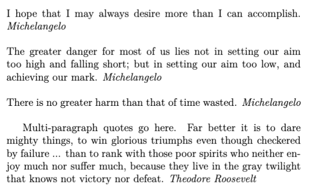
\begin{quote}
  I hope that I may always desire more than I can accomplish. \emph{Michelangelo}

  The greater danger for most of us lies
  not in setting our aim too high and falling short;
  but in setting our aim too low, and achieving our mark. \emph{Michelangelo}

  There is no greater harm than that of time wasted. \emph{Michelangelo}
\end{quote}
\begin{quotation}
  Multi-paragraph quotes go here.
  Far better it is to dare mighty things,
  to win glorious triumphs even though checkered by failure ...
  than to rank with those poor spirits who neither enjoy much nor suffer much,
  because they live in the gray twilight that knows not victory nor defeat.
  \emph{Theodore Roosevelt}
\end{quotation}
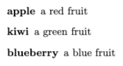
Lists
Bulleted lists are created with \item commands
inside the “itemize” environment. For example:
\begin{itemize}
  \item red
  \item green
  \item blue
\end{itemize}
Numbered lists are created with \item commands
inside the “enumerate” environment. For example:

\begin{enumerate}
  \item red
  \item green
  \item blue
\end{enumerate}
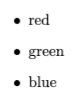
Description lists are created with \item commands
inside the “description” environment. For example:
\begin{description}
  \item[apple] a red fruit
  \item[kiwi] a green fruit
  \item [blueberry] a blue fruit
\end{description}
Lists can be nested up to four levels deep. For example:
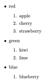
\begin{itemize}
  \item red
    \begin{enumerate}
      \item apple
      \item cherry
      \item strawberry
    \end{enumerate}
  \item green
    \begin{enumerate}
      \item kiwi
      \item lime
    \end{enumerate}
  \item blue
    \begin{enumerate}
      \item blueberry
    \end{enumerate}
\end{itemize}
Code Listings
The listings package renders programming code source code.
It can render code in many programming languages including
Bash, C, C++, Go, Haskell, Java, JavaScript, Lisp, Lua, Matlab,
Perl, PHP, Python, R, Ruby, Rust, Scheme, SQL, and Swift.
It can also render many markup languages including
CSS, HTML, JSON, LaTeXTeX, XML, and YAML.
See the \lstdefinelanguage command that adds support for more languages.
For example:
\usepackage{listings}
\usepackage[dvipsnames]{xcolor} % dvipsnames gives 68 more predefined colors.
...
\lstset{backgroundcolor=\color{Apricot}, numbers=left}
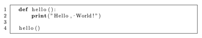
\begin{lstlisting}[caption={Hello World code}, frame=single, frameround=tttt, language=Python]
def hello():
print("Hello, World!")
hello()
\end{lstlisting}
To include a page containing a list of code listing
where each line is a link to a code listing,
add the \lstlistoflisting command.
This causes LaTeX to create a .lol file
that is used to render the list of listings pages.
The \lstlistoflisting command typically appears after the table of contents.
To include this page in the table of contents,
add the following after the \lstlistoflisting command
where “Code Listings” can be any page title:
\addcontentsline{toc}{chapter}{Code Listings}
A better option is to use the minted package.
This uses the Python library Pygments to format source code.
The supported languages are listed at Pygment Languages.
The minted package requires access to the pygentize command.
To install that in macOS, enter brew install pygments.
The following is an example of rendering Smalltalk code:
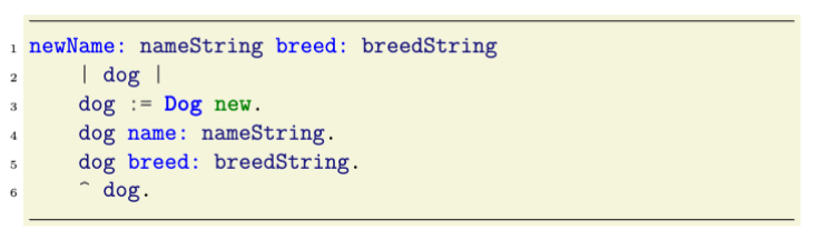
\begin{listing}[H] % see "here" in Figures section
  \begin{minted}[bgcolor=Beige, frame=lines, framesep=3mm, linenos, numbersep=3pt]{smalltalk}
newName: nameString breed: breedString
    | dog |
    dog := Dog new.
    dog name: nameString.
    dog breed: breedString.
    ^ dog.
  \end{minted}
  \caption{My Smalltalk code} % see "\caption" in Figures section
\end{listing}
Listings with a caption are automatically numbered. The sequence of listing numbers is independent from the numbering of figures and tables.
Horizontal Rules
To draw a horizontal line across the page, use \hrule.
Links and URLs
To render a URL in a monospace font, use the \texttt command.
For example, \texttt{https://mvolkmann.github.io/blog/}.
The URL will not be clickable.
To render a clickable URL, include the hyperref package
and use the \url or \href command.
The \url command renders the URL.
The \href command renders alternate text instead of the URL.
For example:
\usepackage{hyperref}

% linkcolor is used for internal links
% like those in the table of contents and index.
% urlcolor is used for external links
% like those created with the \url and \href commands.
% To use additional color names, include the following in the preamble:
% \usepackage[dvipsnames, svgnames]{xcolor}
% dvipsnames are described at
% https://en.wikibooks.org/wiki/LaTeX/Colors#The_68_standard_colors_known_to_dvips
% svgnames are described at https://www.latextemplates.com/svgnames-colors.
\hypersetup{colorlinks=true, linkcolor=DarkBlue, urlcolor=FireBrick}
...
\url{https://mvolkmann.github.io/blog/}

\href{https://mvolkmann.github.io/blog/}{My Blog}
Verbatim Text
Text can be rendered verbatim in order to:
- begin on a new line
- print in a monospace font
- honor all line breaks
- avoid interpreting anything in the text as LaTeX commands
- begin the content that follows on a new line
For short text, use the \verb command
with the text delimited by vertical bars (pipes).
Why aren’t curly braces used instead?
For example:
\verb|This text will be rendered verbatim|
For long text, use a verbatim environment.
For example:
\begin{verbatim}
This haiku will be rendered verbatim.

Out of memory.
We wish to hold the whole sky,
but we never will.
\end{verbatim}
Columns
Rendering content in multiple columns
is not supported by the pdflatex command.
The xelatex or lualatex command must be used instead.
To render an entire document with two columns,
add the twocolumn option to the document class.
For example:
\documentclass[twocolumn]{article}
To render a section of content in multiple columns,
use the multicol package. For example:
\usepackage{multicol}
...
\begin{multicols}{2}
The content to appear in multiple columns goes here.
\end{multicols}
The multicols environment is distinct from
the \multicolumn command that is used in tables.
The commands \onecolumn and \twocolumn can be
used to switch between those options, but for me the \twocolumn command
produces columns that overlap slightly and spill outside the areas
where the text should be contrained.
The multicol package demonstrated above seems to produce better results.
To change the horizontal space between columns,
using the \setlength and \columnsep commands.
For example:
\setlength{\columnsep}{1cm}
To add vertical lines between the columns,
using the \setlength and \columnseprule commands.
For example:
\setlength{\columnseprule}{2pt}
Splitting Documents
A .tex file can include the contents of other .tex files.
This enables breaking a large document into smaller documents
that can be edited independently, such as each chapter of a book.
It also sharing the definitions of custom commands and environments
with multiple documents.
The documents being included should not contain a preamble section
or the \begin{document} and \end{document} commands.
The commands \input and \include can be both be used for this purpose.
Both commands take a file name that is assumed
to be in the same directory as the main .tex file.
It is not necessary to include the .tex file extension.
The \include command starts its content on a new page and
begins a new page before rendering the content that follows.
This command cannot be nested,
so included files cannot use the \include command.
For example:
\include{other-file-name}
To temporarily avoid rendering the content of files included with \include,
add the \includeonly command in the preamble
with an argument that lists the file names to include.
This will not change the numbering of the chapters and sections that follow.
For example:
\includeonly{preface, chapter2}
The \input command start its content where it appears and
does not force a new page before or after the included content.
This command can be nested, so included files can use the \input command.
For example:
\input{other-file-name}
To temporarily avoid rendering the content of files included with \input,
comment out those lines.
This will change the numbering of the chapters and sections that follow.
Boxes
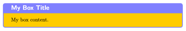
The tcolorbox package renders a colored box with
a title bar at the bottom and content below.
The coloframe option specifies the border color
and background color of the title area.
The colback option specifies the background color of the content area.
Color names can be followed with ! and
a number that specifies a percentage opacity.
For example, red!30 means red with an opacity of 30%.
To specify a second color that should mixed with the first,
add another ! after the percentage value followed by another color.
For example, red!30!yellow means 30% red and 70% yellow.
For example:
\usepackage{tcolorbox}
...
\begin{tcolorbox}[
  title=\large\textsf{\textbf{My Box Title}},
  colback=red!20!yellow,
  colframe=blue!50
]
  My box content.
\end{tcolorbox}
Figures
The figure environment creates floating content,
meaning the compiler can choose its location.
The content is typically a graphical element like an image or diagram,
but it can be anything, include plain text.
A caption can be added above or below the figure content
by adding a \caption{some caption} command.
Figures with a caption are automatically numbered.
The sequence of figure numbers is independent from
the numbering of listings and tables.
To prevent numbering, use the caption package and the \caption* command.
A label can be applied to a figure to enable adding references to the figure.
This is done by adding a \label{some-label} command
in a figure environment.
By default, the compiler will choose the location of the element,
placing it at the top of the current page, bottom of the current page,
or on a new page containing only figures and tables.
The float package adds support for overriding the compiler
with the following options:
- The “h” option tells the compiler to place the item “here” if possible.
- The “H” option tells the compiler to absolutely place the item “here”. The option “!h” is somewhat equivalent.
- The “t” option moves the item to the top of the page.
- The “b” option moves the item to the bottom of the page.
The same options can be used to control the placement of tables.
The following example renders an image that is scaled to be 3 inches wide.
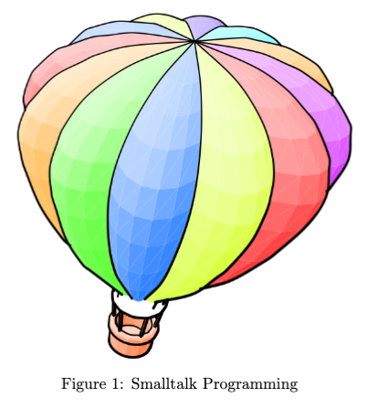
\begin{figure}[H]
  \centering
  \includegraphics[width=3in]{smalltalk-balloon}
  \caption{Smalltalk Programming}
  \label{smalltalk-balloon}
\end{figure}
Any number of references to this figure can occur elsewhere in the document. For example:

My favorite programming language is Smalltalk \ref{smalltalk-balloon}.
To include a page containing a list of figures
where each line is a link to a figure,
add the \listoffigures command.
This causes LaTeX to create a .lof file
that is used to render the list of figures pages.
To include this page in the table of contents,
add the following after the \listoffigures command
where “Images” can be any page title:
\addcontentsline{toc}{chapter}{Images}
References
To reference a figure, listing, or table
that is labeled with \label{some-label},
use the \ref{some-label} command.
If the hyperref package is included with \usepackage{hyperref},
this will output a hyperlink to the item using its assigned number.
Only the number will be output, so consider adding
the word “figure”, “listing”, or “table” before this.
For example, “See table \ref{dog-table}.”
To instead output a page number reference to a figure, listing, or table
that is labeled with \label{some-label},
use the \pageref{some-label} command.
If the hyperref package is included with \usepackage{hyperref},
this will output a hyperlink to the item using its page number.
Only the number will be output, so consider adding
the word “page” before this.
For example, “See page \pageref{dog-table}.”
Images
To include images, use the graphicx package.
Use the \includegraphics command, specifying a file name.
It is not necessary to include the file extension.
The image file must reside in the same directory as the .tex file.
The supported image formats include JPEG (.jpg or .jpeg),
PNG (.png), and PDF (.pdf).
Surrounding the image with a “figure” enables adding a caption which will be automatically numbered along with other figures and can be placed above or below the image.
For example:
\usepackage{float, graphicx}
...
% non-figure image - caption specified with an argument
\includegraphics[width=3in]{Smalltalk-balloon}{Smalltalk Programming}
...
% figure image - caption specified in its own command
\begin{figure}[H]
  \centering % horizontally centers image (caption always is centered)
  \includegraphics[width=3in]{Smalltalk-balloon}
  \caption{Smalltalk Programming}
\end{figure}
In the example above we specified the image width.
Any supported unit of measure can be used.
These include cm (centimeters), em (width of M), ex (height of x),
in (inches), and pt (points).
To scale an image so its width matches that of the current text area,
use \textwidth for the width value.
This can be preceded by a percentage.
For example, [width=0.7\textwidth].
To scale an image so its width matches that of the current line,
use \linewidth for the width value.
Instead of specifying a width, a height (a measure like width)
or scale (a number treated as a percentage) can be specified.
Math Mode
Mathematical equations are specially formatted when in math mode. This includes making variables names italicized and properly formatting fractions, subscripts, supercripts, and more.
There are two kinds of math mode, inline and display. Inline math mode renders mathematical text inline with other content. Display math mode renders mathematical text on its own line, separated from surrounding content and horizontally centered by default.
To use inline math mode, surround content by single dollar signs,
\( and \), or \begin{math} and \end{math}. For example:

The Pythagorean theorem states that
for a triangle with sides of length $a$ and $b$
and hypotenuse of length $c$, $a^2 + b^2 = c^2$.
Fractions are rendered using the \frac (small) and \dfrac (large) commands.
When in display mode (inside double dollar signs), both are rendered large,
so \dfrac is only needed in inline math mode.
For both commands, the numerator and denominator
are specified in their own pair of curly braces.
For example:
Inline fractions can be small like $\frac{x}{y}$ or large like $\dfrac{x}{y}$.
To use display math mode, surround content by double dollar signs,
\[ and \], or \begin{displaymath} and \end{displaymath}.
Each formula should appear on its own line
and all but the last should end in \\.
LaTeX will not break a long formula over multiple lines,
so each formula must fit on one line.
The Pythagorean theorem states that
for a triangle with sides of length $a$ and $b$
and hypotenuse of length $c$, $a^2 + b^2 = c^2$.

The following is the formula calculates the velocity $v$
that an object will be travelling after falling over time $t$
given acceleration due to gravity of $g$ (9.8 $m/s^2$ on Earth).

$$ v = \frac{1}{2} g t^2 $$
A vertically centered dot represents multiplication and can add clarity. In the expression $ 2xy^2 $ it is clear that $2$, $x$, and $y^2$ are to be multiplied. In this case adding dots between the terms doesn’t add clarity. On the other hand, $23$ represents a single number, not multiplying $2$ and $3$. In this case it is appropriate to write \verb|$2 \cdot 3| which is rendered as follows:

The equation environment is like the displaymath environment,
but it adds numbers in parentheses to the right of equations
to identify them. For example:
\begin{equation}
    area = width \cdot height
\end{equation}
\begin{equation}
    area = \frac{1}{2} \cdot base \cdot height
\end{equation}
All roots, square and otherwise, are rendered with the \sqrt command.
For example:
$$ \sqrt{25} = 5 $$
$$ \sqrt[3]{8} = 2 $$
$$ x = \frac{-b \pm \sqrt{b^2 - 4ac}}{2a} $$
The following are additional examples of using math mode:
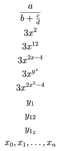
$$ \frac{a}{b + \frac{c}{d}} $$ % nested fractions
$$ 3x^2 $$ % single-character superscript
$$ 3x^{12} $$ % multi-character superscript (requires curly braces)
$$ 3x^{2x - 4} $$ % more complex exponent
$$ 3x^{y^z} $$ % multiple levels of exponents
$$ 3x^{2x^5 - 4} $$ % more complex multiple levels of exponents
$$ y_1 $$ % single-character subscript
$$ y_{12} $$ % multi-character subscript (requires curly braces)
$$ y_{1_2} $$ % multiple levels of subscripts
$$ x_0, x_1, \ldots, x_n $$ % sequence of subscripted variables with ellipsis
The \left and \right commands are used to make grouping characters
like parentheses, square brackets, curly braces, and vertical bars
have a height that matches their content.
The following example demonstrates what is rendered
without and with those commands.
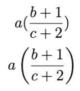
$$ a (\frac{b + 1}{c + 2}) $$
$$ a \left(\frac{b + 1}{c + 2}\right) $$
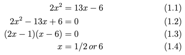
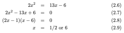
To align equal signs when showing the solution to an equation,
use the amsmath package, wrap the steps in an align environment,
preceded each = with &, and end each line with \\.
It is not necessary to have any text before the equal sign.
For example:
\begin{align}
f(x) &= x^2 - 20x + 6 + 7x + x^2 \\
     &= 2x^2 - 13x + 6 \\
     &= (2x - 1)(x - 6)
\end{align}
\begin{align}
2x^2 &= 13x - 6 \\
2x^2 - 13x + 6 &= 0 \\
(2x - 1)(x - 6) &= 0 \\
x &= 1/2 \,or\, 6
\end{align}
The steps will be numbered by default.
To prevent numbering, use align* in place of align.
The following formatting commands can only be used in math mode:
\mathbf{This is bold.}
\mathit{This is italic.}

\mathrm{This uses a Roman font.}
\mathsf{This uses a sans serif font.}
\mathtt{This uses a typewriter font.} % monospace

\overline{This has a horizontal line above.}
\overbrace{This has a horizontal brace above.}
\underbrace{This has a horizontal brace below.}
The \underline command can be used in any mode
to draw a horizontal line below its argument.
To add text above an \overbrace, use a superscript.
To add text below an \underbrace, use a subscript.
For example:
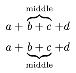
$$
  a + \overbrace{b + c}^{\textup{middle}} + d
$$
$$
  a + \underbrace{b + c}_{\textup{middle}} + d
$$
The following examples demonstrate rendering limits, sums, and integrals:
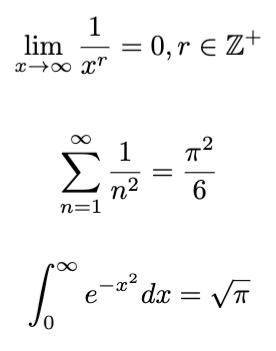
$$ \lim_{x \to \infty} \frac{1}{x^r} = 0, r \in \mathbb{Z^+} $$
$$ \sum_{n=1}^\infty \frac{1}{n^2} = \frac{\pi^2}{6} $$
$$ \int_0^\infty e^{-x^2} dx = \sqrt{\pi} $$
There are commands for standard math functions
that can only be used in math mode.
They prevent function names from being rendered in italics like variable names.
Examples include \sin, \cos, \tan, \ln, \log, and \gcd.
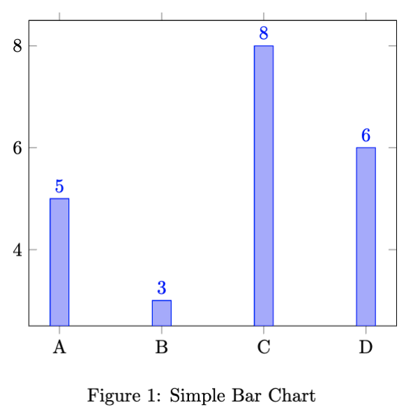
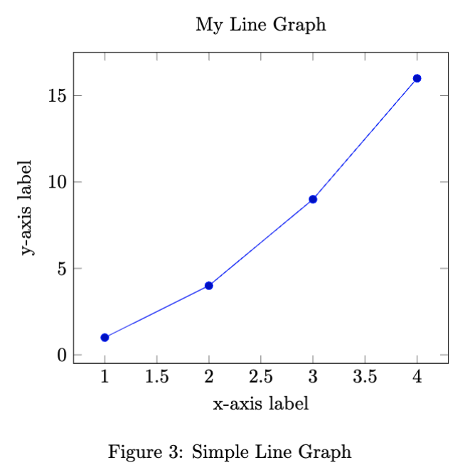
Charts
LaTeX can render many kinds of charts. The following document demonstrates several of these.
\documentclass{article}
\usepackage{pgf-pie}
\usepackage{pgfplots}

\pgfplotsset{compat=1.18}
\usepgfplotslibrary{fillbetween}

\begin{document}
\begin{figure}
  \centering
  \begin{tikzpicture}
    \begin{axis}[
        ybar,
        symbolic x coords={A, B, C, D},
        xtick=data,
        nodes near coords
    ]
      \addplot coordinates {(A, 5) (B, 3) (C, 8) (D, 6)};
    \end{axis}
  \end{tikzpicture}
  \caption{Simple Bar Chart}
\end{figure}
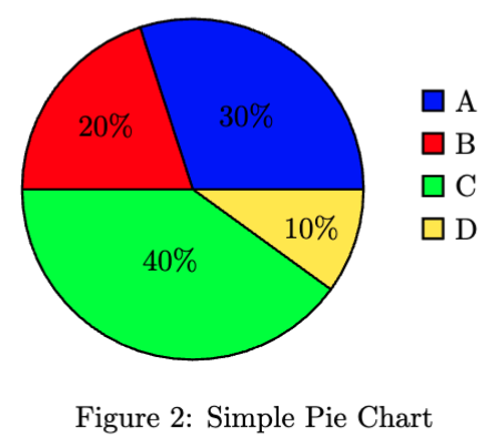
\begin{figure}
  \centering
  \begin{tikzpicture}
    \pie[
      text=legend,
      radius=2,
      color={blue, red, green, yellow}
    ]{
        30/A,
        20/B,
        40/C,
        10/D
    }
  \end{tikzpicture}
  \caption{Simple Pie Chart}
\end{figure}
% TODO: How can this be modified to fill the area below the line?
\begin{figure}
  \centering
  \begin{tikzpicture}
    \begin{axis}[
      title={My Line Graph},
      xlabel={x-axis label},
      ylabel={y-axis label}
    ]
      \addplot coordinates {
        (1, 1)
        (2, 4)
        (3, 9)
        (4, 16)
     }; % semicolon is really required
    \end{axis}
  \end{tikzpicture}
  \caption{Simple Line Graph}
\end{figure}
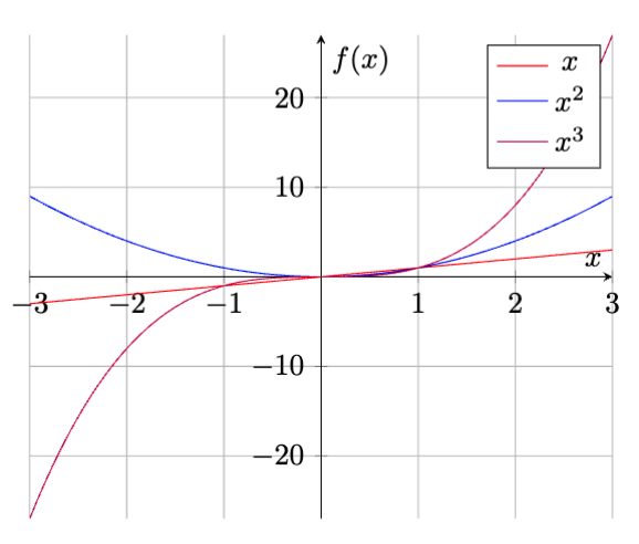
\begin{figure}
  \centering
  \begin{tikzpicture}
    \begin{axis}[
        axis lines = center,
        grid = both,
        xlabel = \(x\),
        ylabel = {\(f(x)\)},
    ]
      \addplot [domain=-3:3, samples=100, color=red]
      {x};
      \addlegendentry{\(x\)}

      \addplot [domain=-3:3, samples=100, color=blue]
      {x^2};
      \addlegendentry{\(x^2\)}

      \addplot [domain=-3:3, samples=100, color=purple]
      {x^3};
      \addlegendentry{\(x^3\)}
    \end{axis}
  \end{tikzpicture}
\end{figure}
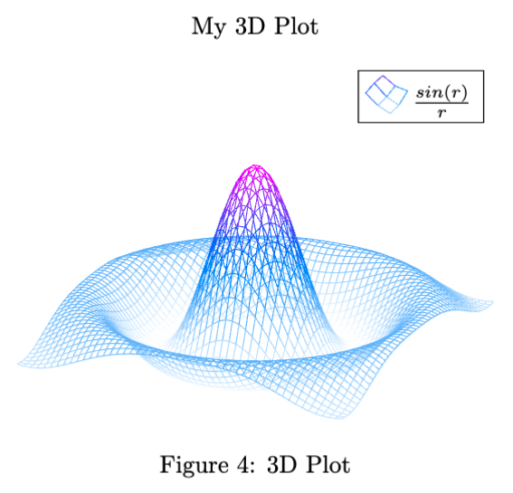
% This takes as long time to render (around 15 seconds)!
\begin{figure}
  \centering
  \begin{tikzpicture}
    \begin{axis}[
        title={My 3D Plot},
        hide axis,
        colormap/cool,
    ]
      \addplot3[
          mesh,
          samples=50,
          domain=-8:8,
      ]
      {sin(deg(sqrt(x^2+y^2)))/sqrt(x^2+y^2)};
      \addlegendentry{\(\frac{sin(r)}{r}\)}
    \end{axis}
  \end{tikzpicture}
  \caption{3D Plot}
\end{figure}

\end{document}
Dots
Dot commands render an ellipsis in different orientations. Simply typing three periods does not result in the correct spacing for an ellipsis.
The following examples demonstrate the dot commands:
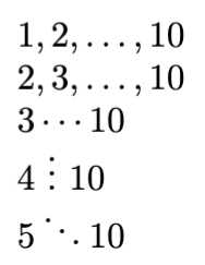
$ 1, 2, \dots, 10 $ \\ % horizontal dots
$ 2, 3, \ldots, 10 $ \\ % lower horizontal dots
$ 3 \cdots 10 $ \\ % vertically centered horizontal dots
$ 4~ \vdots ~10 $ \\ % vertical dots; ~ ("tie") and is like   in HTML
$ 5 \ddots 10 $ \\ % diagonal dots
The commands \dots, \ldots, and \vdots can be used in any mode.
The commands \cdots and \vdots can only be used in math mode.
Arrays
Arrays render values in rows and columns of math formulas
and can only be used in math mode.
For rows and columns of text items, use the tabular environment.
The array environment has a required parameter that indicates
the number of columns and the horizontal alignment of each.
For example, the following displays some formulas related to circles.
The argument ll indicates that there are
two columns and both are left-aligned.
Use c for columns that are centered
and r for columns that are right-aligned.
The \textup command is used here to prevent words from being
treated as variables and therefore being printed in italics.
$$
  \begin{array}{ll}
    \textup{diameter}      & 2r      \\
    \textup{circumference} & 2 \pi r \\
    \textup{area}          & \pi r^2 \\
  \end{array}
$$
To place delimiters such as vertical bars, parentheses, square brackets,
or curly braces on the left and right sides of an array,
use the \left and \right commands.
The delimeters will have the full height the associated array.
For example:
\left| ... \right|
\left( ... \right)
\left[ ... \right]
\left\{ ... \right\} % curly braces must be escaped
The \left and \right commands must be used as a pair.
To place a delimiter only on one side,
specify a period for the other side to make it invisible.
For example, \left. ... \right\} renders
no delimeter on the left side and a curly brace on the right side.
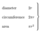
$$
  \left.
  \begin{array}{ll}
    \textup{diameter}      & 2r      \\
    \textup{circumference} & 2 \pi r \\
    \textup{area}          & \pi r^2 \\
  \end{array}
  \right\}
$$
The eqnarray environment creates a three-column array
where the first column contains the left sides of equations,
the last column contains the right sides of equations,
and the center column describes the relationships
between the left and right sides (usually =).
The equation described in each row is numbered.
For example:
\begin{eqnarray}
  2x^2 & = & 13x - 6 \\
  2x^2 - 13x + 6 & = & 0 \\
  (2x - 1)(x - 6) & = & 0 \\
  x & = & 1/2 \textup{ or } 6
\end{eqnarray}
This environment automatically uses math mode for its contents and will output the following error messages if embedded in math mode:
LaTeX Error: \begin{document} ended by \end{eqnarray}
Missing $ inserted
Display math should end with $$
To avoid rendering equation numbers, use eqnarray*.
If an equation is too long to fit on a single line,
use the \lefteqn command to allow using multiple lines.
Matrices
Matrices are rendered with matrix environment. These include the following:
bmatrix: square bracketsBmatrix: curly bracesmatrix: no bracketspmatrix: parenthesesvmatrix: single vertical barsVmatrix: double vertical bars
For example, the following is the formula for rotating a 3D point about the origin in the x/y plane. In math mode a single quote renders a prime symbol, two single quotes render a double prime, and so on.
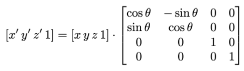
$$
[x' \, y' \, z' \, 1]
=
[x \, y \, z \, 1] \cdot
\begin{bmatrix}
    \cos\theta & -\sin\theta & 0 & 0 \\
    \sin\theta & \cos\theta & 0 & 0 \\
    0 & 0 & 1 & 0 \\
    0 & 0 & 0 & 1 \\
\end{bmatrix}
$$
Tables
To create a table, use the \begin{tabular}{columns} command.
This can be used in any mode, unlike the array environment
which can only be used in math mode.
“columns” is replaced by text that specifies:
- the number of columns
- whether they should be left-aligned (
l), centered (c), or right-aligned (r) - whether there should be vertical borders before the columns, between the columns, and after the columns
For example, \begin{tabular}{|c|lr|} creates a table with three columns.
The first column is centered, the second is left-aligned, and the last is right-aligned.
There will be vertical lines before the first and second columns,
and after the last column, that extent the entire height of the table.
The table rows are specified with content that follows
up to the \end{tabular} command.
The cells of each row are separated by the & character.
The end of each row is marked by \\.
To add horizontal lines before and/or after a row, add the \hline command.
To add double lines, such as below the heading row,
add two \hline commands.
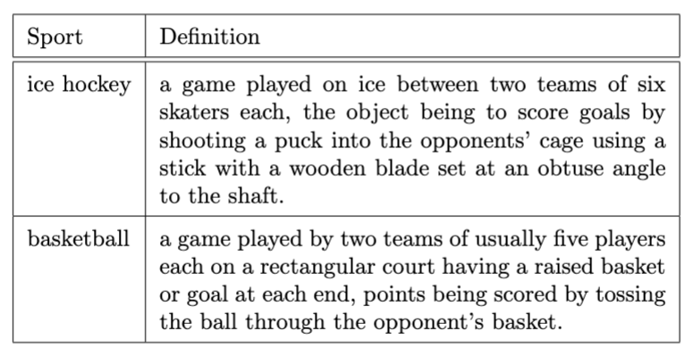
The following example creates a table describing dogs.
It uses the \textbf command is used to make the column headings bold.
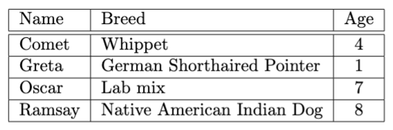
\begin{tabular}{|l|l|c|}
  \hline
  \textbf{Name} & \textbf{Breed} & \textbf{Age} \\
  \hline\hline
  Comet & Whippet & 4 \\
  \hline
  Greta & German Shorthaired Pointer & 1 \\
  \hline
  Oscar & Lab mix & 7 \\
  \hline
  Ramsay & Native American Indian Dog & 8 \\
  \hline
\end{tabular}
The command \def\arraystretch adds padding to table cells.
To add padding to the table cells of a specific table,
add the following in the table envirionment:
\def\arraystretch{1.5}
To add padding to the table cells of all tables, add the following in the preamble:
\renewcommand{\arraystretch}{1.5}
To change the color and thickness of the table cell borders, add the following in the preamble:
\arrayrulecolor{red}
\setlength{\arrayrulewidth}{1mm}
To change the background color of a single row,
add \rowcolor{color} before its data.
To change the background color of a single cell,
add \cellcolor{color} before its data.
For example, the following makes the background color of a row pale yellow, and makes the second cell be pink:
\rowcolor{yellow!50}Comet & \cellcolor{red!20}Whippet & 4 \\\
To alternate the background colors of all rows except the first,
which typically contains column headings,
add the following before the beginning of the tabular environment:
To specify the background color for all cells in a column, including the cell in the header row:
-
Define a new column type in the preamble.
% Column type "i" (for important) is red and centered. \newcolumntype{i}{>{\columncolor{red!20}}c} -
Use the new column type in place of the built-in types that include
l,c, andr.\rowcolors{2}{odd-row-color}{even-row-color}
A caption can be added above or below the table content
by adding a \caption{some caption} command.
The caption will be automatically numbered by default.
To prevent numbering, use the caption package and the \caption* command.
A label can be applied to a table to enable adding references to the table.
This is done by adding a \label{some-label} command
in a table environment.
To reference the table, use the \ref{some-label} command.
For example:
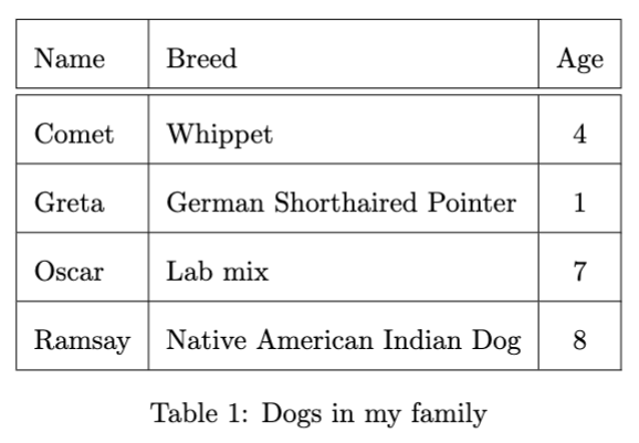
\usepackage{float}
...
\begin{table}[H] % absolutely positions table here
  \centering % centers table on page
  \def\arraystretch{2} % adds padding inside cells
  \begin{tabular}{|l|l|c|}
    \hline
    Name & Breed & Age \\
    \hline\hline
    Comet & Whippet & 4 \\
    \hline
    Greta & German Shorthaired Pointer & 1 \\
    \hline
    Oscar & Lab mix & 7 \\
    \hline
    Ramsay & Native American Indian Dog & 8 \\
    \hline
  \end{tabular}
  \caption{Dogs in my family}
  \label{dog-table}
\end{table}
...
Do you like dogs? \ref{dog-table}
Tables with a caption are automatically numbered. The sequence of table numbers is independent from the numbering of listings and figures.
To include a page containing a list of tables
where each line is a link to a table,
add the \listoftables command.
This causes LaTeX to create a .lot file
that is used to render the list of tables pages.
To include this page in the table of contents,
add the following after the \listoffiguures command
where “Tables” can be any page title:
\addcontentsline{toc}{chapter}{Tables}
The [H] option can be specified on a table environment,
but not on a tabular environment.
Text in a table cell can contain paragraphs of text that wrap to multiple lines. For example:
\begin{table}[H]
  \def\arraystretch{1.5} % adds padding inside cells
  \begin{tabular}{|l|p{3in}|} % note use of p with a specified width
    \hline
    Sport & Definition \\
    \hline\hline
    ice hockey & a game played on ice between two teams of six skaters each, the object being to score goals by shooting a puck into the opponents' cage using a stick with a wooden blade set at an obtuse angle to the shaft. \\
    \hline
    basketball & a game played by two teams of usually five players each on a rectangular court having a raised basket or goal at each end, points being scored by tossing the ball through the opponent's basket. \\
    \hline
  \end{tabular}
\end{table}
The table below demonstrates the following:
- cells that span multiple columns
- cells that span multiple rows
- cells that span both multiple columns and multiple rows
The \multicolumn command does not require an additional package.
It takes three arguments that describe the number of columns to span,
the horizontal positioning of its content (l, c, or r),
and the content.
The second argument can also contain vertical bars to indicate
borders to be drawn on the left and/or right side of the content.
The \multirow command is defined in the multirow package.
The \cellcolor command is defined in the colortbl package
and requires the xcolor package.
When the \cellcolor command is applied to a cell that spans more than one row,
only the first row is affected. Is this a bug?
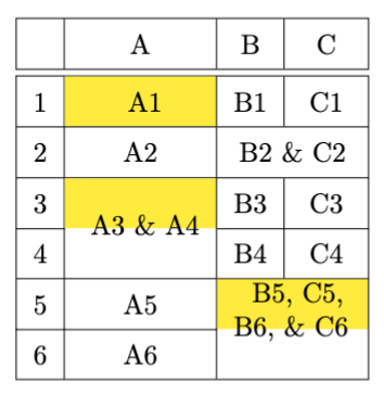
\usepackage{colortbl, multirow, xcolor}
...
\def\arraystretch{1.5} % adds padding inside cells
\begin{tabular}{|c|c|c|c|}
  \hline
  & A & B & C \\
  \hline\hline
  1 & \cellcolor{yellow} A1 & B1 & C1 \\
  \hline

  2 & A2 & \multicolumn{2}{c|}{B2 \& C2} \\
  \hline

  3 & \multirow{2}{*}{\cellcolor{yellow} A3 \& A4} & B3 & C3 \\
  \cline{1-1} \cline{3-4} % Draw cell lines below cells 1, 3, and 4.

  4 & & B4 & C4 \\
  \hline

  5 & A5 & \multicolumn{2}{c|}{
    \multirow{2}{1.5cm}{
      \cellcolor{yellow} B5, C5, B6, \& C6
    }
  } \\
  \cline{1-2} % Draw cell lines below cells 1 and 2.

  6 & A6 & \multicolumn{2}{c|}{} \\
  \hline
\end{tabular}
TODO: When I use \cellcolor in a \multirow, it only colors the first row.
TODO: Am I doing something wrong in this simple example?
TODO: I posted this question here: https://www.youtube.com/watch?v=xyZtxfMsD38
\begin{tabular}{|c|c|c|}
  \hline
  1 & \multirow{2}{*}{\cellcolor{yellow} 2 and 6} & 3 \\
  \cline{1-1} \cline{3-3}
  5 & & 7 \\
  \hline
\end{tabular}
Tables created with the tabular environment
cannot span across page boundaries.
The longtable package supports this and provides an option
for the table headings and footers to be repeated on each page.
For example:
\usepackage{longtable}
...
\begin{longtable}{|l|c|l|}
  \hline
  Description & Symbol & Command \\
  \hline\hline
  \endhead % marks the end of the heading rows
  checkmark & $\checkmark$ & \verb|\checkmark| \\
  circle & $\circ$ & \verb|\circ| \\
  club suit & $\clubsuit$ & \verb|\clubsuit| \\
  ...
  \hline
\end{longtable}
Also see the commands \endfirsthead, \endlastfoot, and \endfoot.
Other packages that support rendering tables include
tabu, tabularx, and tabulary.
Scaling, Resizing, and Rotating
The graphicsx package defines the following commands (and more):
\scalebox- argument is a constant scale factor\resizebox- arguments are width and height\rotatebox- argument is angle in degrees
For example:

\scalebox{3}{TEST}

\resizebox{1in}{1.5in}{TEST}

\rotatebox{45}{TEST}
picture Environment
The picture environment supports drawing basic diagrams containing
lines, arrows, rectangles, circles, and curves.
Rectangles can be solid or dashed, and they can have square or rounded corners.
Slanted lines, not horizontal or vertical, are drawn using characters from a special font. This limits the accuracy of the line lengths and their slope.
The following example defines several custom commands. Some of them are used as variables in other commands.
The \framebox command takes an optional argument that specifies
where in the box its contents should be rendered.
The location is specified with the following letters
which can be used alone or in a pair:
- l for left
- r for right
- t for top
- b for bottom
The \put command sets the reference point
for the drawing command that follows.
For lines and arrows, the reference point is its starting point.
For shapes like rectangles, ovals, and circles,
the reference point is its center.
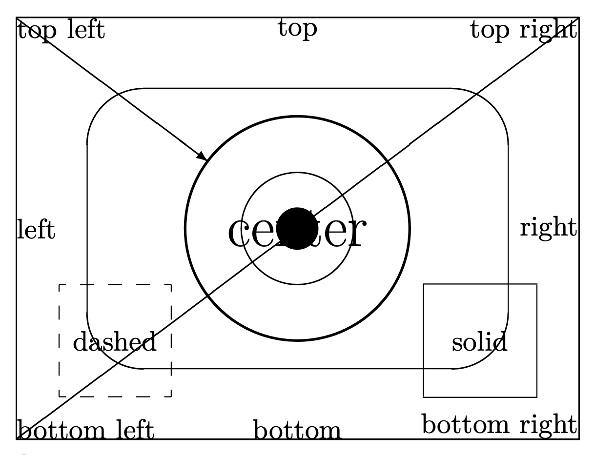
\def\myWidth{200}
\def\myHeight{150}
\newcommand{\myHalfWidth}{\dimexpr\myWidth pt/2\relax}
\newcommand{\myHalfHeight}{\dimexpr\myHeight pt/2\relax}
\def\myDiameter{40}
\def\putOrigin{\put(0, 0)}
\def\putCenter{\put(\myHalfWidth, \myHalfHeight)}
\def\myFramebox{\framebox(\myWidth, \myHeight)}
\begin{picture}(\myWidth, \myHeight)
    \putOrigin{\myFramebox[tl]{top left}}
    \putOrigin{\myFramebox[t]{top}}
    \putOrigin{\myFramebox[tr]{top right}}
    \putOrigin{\myFramebox[l]{left}}
    % Centers text by default.
    \putOrigin{\myFramebox{\huge{center}}}
    \putOrigin{\myFramebox[r]{right}}
    \putOrigin{\myFramebox[b]{bottom}}
    \putOrigin{\myFramebox[bl]{bottom left}}
    \putOrigin{\myFramebox[br]{bottom right}}

    % Slopes must be defined with two integers
    % that form a fraction in its simplest form.
    % So 4/3 is valid, but 8/6 is not.
    \putOrigin{\line(4, 3){\myWidth}} % diagonal line with slope 4/3
    \put(0, \myHeight){\vector(4, -3){68}} % arrow with slope 4/-3, not -4/3

    % Supported circle sizes include 1-41.
    % To get larger circles, combine the use of
    % \scalebox defined in the graphicx package.
    % It specifies the number of times larger to make its argument,
    % so \scalebox{1} doubles the size.
    \putCenter{\circle*{\myDiameter}} % filled circle
    \putCenter{\scalebox{1}{\circle{\myDiameter}}} % hollow circle
    \putCenter{\scalebox{2}{\circle{\myDiameter}}} % hollow circle

    \putCenter{\oval(150, 100)} % oval

    \put(15, 15){\dashbox{5}(40, 40){dashed}} % dashed rectangle
    \put(145, 15){\framebox(40, 40){solid}} % solid rectangle
\end{picture}
To draw graph paper grids, use the \graphpaper command
that is defined in the graphpap package.
This takes an optional argument that specifies the grid spacing
with a default value of 10.
That is followed by the coordinates of the lower-left corner
and the width and height.
The following example uses a grid spacing of 15, begins at x = 0, y = 0, has a width of 200 and a height of 150.
\usepackage{graphpap}
...
\graphpaper[15](0,0)(200,150)
Greek Letters
Greek letters are produced using the following commands. There are no commands for Greek letters that are identical to the corresponding Latin letter, Latin letters are used for those.
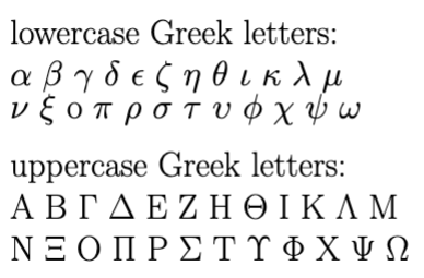
| Name | Lowercase | Uppercase |
|---|---|---|
| alpha | $\alpha$ | A |
| beta | $\beta$ | B |
| gamma | $\gamma$ | $\Gamma$ |
| delta | $\delta$ | $\Delta$ |
| epsilon | $\epsilon$ | E |
| zeta | $\zeta$ | Z |
| eta | $\eta$ | H |
| theta | $\theta$ | $\Theta$ |
| iota | $\iota$ | I |
| kappa | $\kappa$ | K |
| lambda | $\lambda$ | $\Lambda$ |
| mu | $\mu$ | M |
| nu | $\nu$ | N |
| xi | $\xi$ | $\Xi$ |
| omicron | o | O |
| pi | $\pi$ | $\Pi$ |
| rho | $\rho$ | P |
| sigma | $\sigma$ | $\Sigma$ |
| tau | $\tau$ | T |
| upsilon | $\upsilon$ | $\Upsilon |
| phi | $\phi$ | $\Phi$ |
| chi | $\chi$ | X |
| psi | $\psi$ | $\Psi$ |
| omega | $\omega$ | $\Omega$ |
Symbols
Some of the supported symbols are shown in the table below.
The \ddots, \iddots, and \vdots commands
are defined in the mathdots package.
The \frownie and \smiley commands
are defined in the wasysym package.
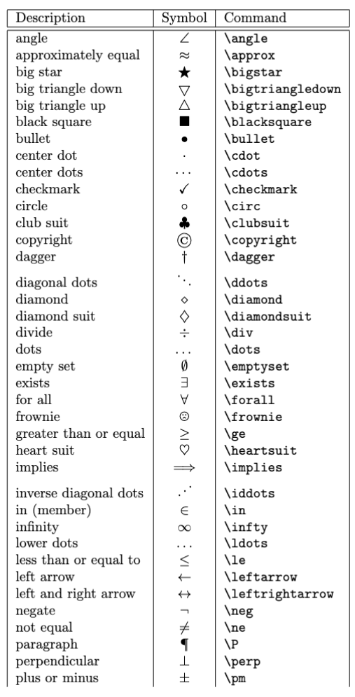
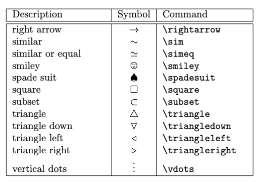
Symbols that represent classes of numbers
are rendered with the \mathbb command.
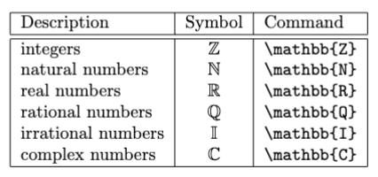
For more, see LaTeX:Symbols.
Document Title, Author, and Date
The preamble can include the \title, \author, and \date commands to
specify information that will be used in a nicely formatted document title.
For example:
\documentclass{article}

% These provide data used by \maketitle.
% They typically appear in the preamble,
% but can appear anywhere before \maketitle.
\title{Server-Driven Web Apps with htmx}
\author{R. Mark Volkmann}
\date{\today} % can omit to default to today
The \date argument can be a specific date.
The \today command provides the current date.
Omitting the \date command will also render the current date.
Use the \maketitle command inside the document to render the
title information in most document classes (not in letter or beamer).
For example:
\begin{document}
\maketitle % generates a title page
...
\end{document}
This renders the following title information:
Table of Contents
A table of contents can be generated for documents that use the
\chapter, \section, \subsection, and \subsubsection commands.
If the package hyperref is included,
the entries in the table of contents will be clickable links.
The \tableofcontents command causes LaTeX to create a .toc file
that is used to render the table of contents pages.
For example:
\documentclass{article}
\usepackage{hyperref}

\begin{document}
\tableofcontents
\listoffigures
\listoftables

\section{Jumping In}
...
\subsection{Choosing a Tech Stack}
...
\subsection{Using htmx Attributes}
...
\subsection{Creating Your First Project}
...
\section{Exploring Server Options}
...
\subsection{Making the Grade}
...
\subsection{Popular Choices}
...
\subsection{Our Choice}
...
\section{Developing Endpoints}
...
\subsection{HTTP Requests}
...
\subsection{HTTP Responses}
...
\subsection{Endpoint Targets}
...
\end{document}
This generates the following table of contents:
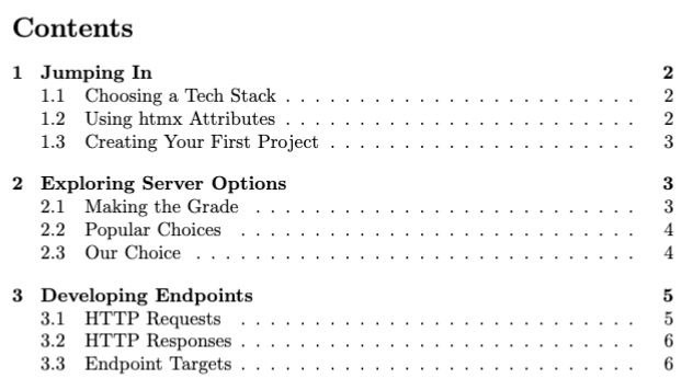
Formatting the Word LaTeX
The word LaTeX is specially formatted with the command \LaTeX
which reneders the following:

Similarly, the word TeX is spacially formatted with \TeX.
Both are typically followed by a backslash and a space to get proper horizontal spacing between it and what follows.
Footnotes
To add numbered footnotes, use the \footnote command.
For example:
Oil that is, black gold, Texas tea.
\footnote{Texas tea is another name for oil.}
This adds a section at the bottom for page like the following:
It also adds a number in square brackets like the following that acts a clickable link to the corresponding footnote.
Appendices
The \appendix command marks the beginning of appendix content.
The following example document demonstrates a book with two appendices
that are included in the table of contents.
\documentclass{book}
\usepackage[toc, page]{appendix}

\title{Server-Driven Web Apps with htmx}
\author{R. Mark Volkmann}

\begin{document}
\maketitle % generates a title page
\tableofcontents % generates table of contents pages

\chapter{Getting Started}
This is the first chapter.

\appendix

\chapter{The Past}
This is the first appendix.

\chapter{The Future}
This is the second appendix.

\end{document}
Bibliography
To add a bibliography pages to a document:
-
Create a
.bibfile, perhaps with the same name as the.texfile that will use it. -
Add directives to the
.bibfile. For example:@book{htmx-volkmann, author = "Volkmann, R. Mark", isbn = "9798888650769", journal = "Pragmatic Bookshelf", pages = "184", publisher = "Pragmatic Bookshelf", title = "Server-Driven Web Apps with Htmx", url = "https://pragprog.com/titles/mvhtmx/server-driven-web-apps-with-htmx/", year = "2024" }Also see the directives @article, @inproceedings, and @misc. Each of these have a different set of required attributes.
-
Add the following commands near the bottom of the
.texfile:\bibliographystyle{plain} \bibliography{some-name} % refers to the file some-name.bibThis causes bibliography pages similar to the following to be generated.
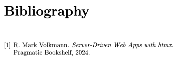
-
Add citations within the document that link to bibliography entries. For example:
Learn about using htmx to build web applications.\cite{htmx-volkmann}This adds a number in square brackets that acts a clickable link to the corresponding bibliography entry.
Index
The imakeidx package generates an index including an alphabetical list
of important words and phrases and the page numbers where they appear.
Each item in the list is a link that can be clicked to scroll to the occurrence.
The following steps achieve this:
-
Include the following in the preamble:
% This needed to include lists of listings, figures, and tables % in the Table of Contents. % The nottoc option tells it to not include the "Contents" page % in the Table of Contents. \usepackage[nottoc]{tocbibind} \usepackage{imakeidx} % This turns index entries into hyperlinks % and must appear before \makeindex. \usepackage{hyperref} % This reads the `.idx` file that is created by `\index` commands. % It creates the `.ind` file % that is read by the `\printindex` command. % It indicates that the index should be included in the TOC. % The number of columns defaults to 2. \makeindex[columns=3, intoc] -
After each occurrence of a word and phrase to be indexed, add
\index{word-or-phrase}. These write to the.idxfile that is read by the\makeindexcommand.To make a word or phrase be a subitem in the index, pass to the
\indexcommand the main and sub index text separated by!. For example,Comet\index{dogs!Comet}The text to be indexed must be duplicated and that is annoying! To avoid duplicating the text, define the following command and replace all occurrences of
word\index{word}with\ind{word}.\newcommand{\ind}[1]{#1\index{#1}} -
Add
\printindexnear the bottom of the document. This reads the.indfile that is generated by the\makeindexcommand. -
Compile by running
pdflatex name.tex. It may be necessary to run this twice.
See the sample content in the “Page Numbering” section.
To add a page range to the index,
mark the beginning of the range with \index{some-term|(}
and mark the end of the range with \index{some-term|)}.
Note the open and close parentheses in these commands.
To reference another index entry instead of supplying a page number,
mark the word or phrase with \index{this-key|see{other-key}}.
Using the \pagenumbering command to switch between
roman and arabic page numbers confuses the \makeindex command,
so unfortunate it seems that cannot be done.
Slide Presentations (beamer)
LaTeX can create PDF-based slide presentations using the “beamer” document class. See the following YouTube videos:
- How I Make Presentations Using LaTeX & Beamer
- LaTeX Tutorial 11: Beamer Slide Presentation
- Overleaf Beamer Guide
The example below demonstrates many beamer features.
It is based on the the first link above
which is to a YouTube video from Dr. Trefor Bazett.
The following screenshot shows the handout pages it generates.
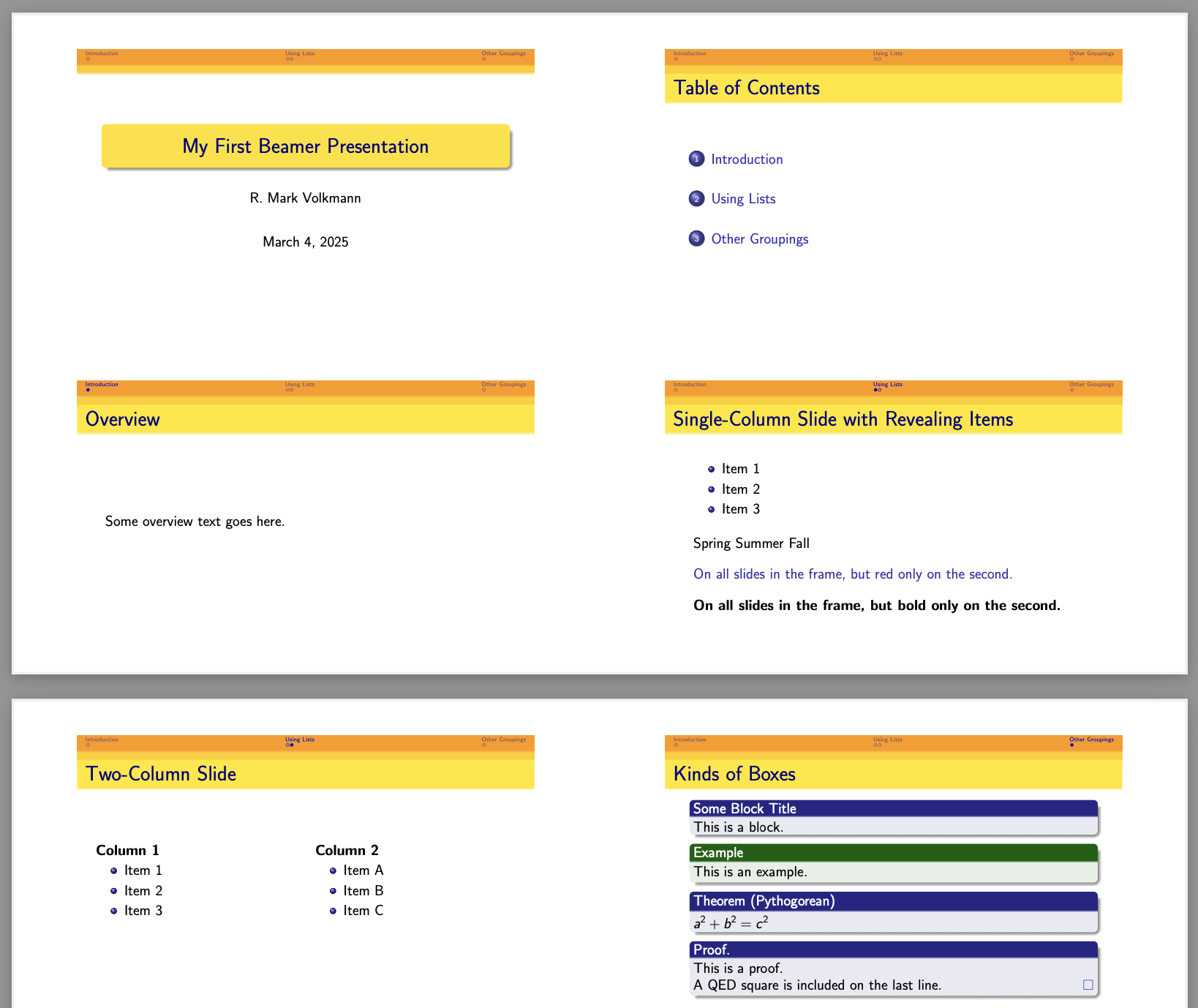
% Specifying 14pt makes the text larger than the default.
% Specifying an aspect ratio of 169 makes it 16 by 9 instead of 4 by 3.
\documentclass[14pt, aspectratio=169, handout]{beamer}

\usepackage[utf8]{inputenc}

% Slide themes are names of cities including
% default, AnnArbor, Antibes, Bergen, Berkeley, Berlin,
% Boadialla, CambridgeUS, Copenhagen, Darmstadt,
% Goettingenm, PaloAlto, Szeged, and Warsaw.
\usetheme{Darmstadt}

% Color themes are names of animals including
% default, beaver, beetle, seahorse, and wolverine.
\usecolortheme{wolverine}

\setbeamertemplate{navigation symbols}{} % hides navigation buttons
\setbeamercovered{transparent} % to faintly see upcoming slide builds

% With these inlines in place, only handout pages are generated.
% Comment them out to see the slides instead.
%\usepackage{pgfpages}
%\pgfpagesuselayout{4 on 1}[border shrink=5mm]

\title{My First Beamer Presentation}
\author{R. Mark Volkmann}
\date{\today}

\begin{document}

\maketitle

\begin{frame}{Table of Contents}
    % This items in this list are links to the first slide in their section.
  \tableofcontents
\end{frame}

\section{Introduction}

\begin{frame}
  \frametitle{Overview}

  Some overview text goes here.
\end{frame}

\section{Using Lists}

% Each slide is described in a frame environment.
\begin{frame}
  \frametitle{Single-Column Slide with Revealing Items}

  \begin{itemize}
    % The items are progressively revealed on separate slides.
    % If the dash after each slide number is removed,
    % only one item will appear on each slide of the frame.
    \item<1-> Item 1
    \item<2-> Item 2
    \item<3-> Item 3
  \end{itemize}

  \vfill
  % These maintain their positions as if all are present,
  % but only one is visible at a time.
  %\onslide<1>{Spring}
  %\onslide<2>{Summer}
  %\onslide<3>{Fall}

  % Only one of these is visible at a time
  % and they render in the same position.
  \only<1>{Spring}
  \only<2>{Summer}
  \only<3>{Fall}

  \vfill
  \alert<2>{On all slides in the frame, but red only on the second.}

  \vfill
  \textbf<3>{On all slides in the frame, but bold only on the second.}
\end{frame}

\begin{frame}
  \frametitle{Two-Column Slide}
  \begin{columns}

    \begin{column}{0.5\textwidth}
      \textbf{Column 1}
      \begin{itemize}
        \item Item 1
        \item Item 2
        \item Item 3
      \end{itemize}
    \end{column}

    \begin{column}{0.5\textwidth}
      \textbf{Column 2}

      \begin{itemize}
        \item Item A
        \item Item B
        \item Item C
      \end{itemize}

    \end{column}
  \end{columns}
\end{frame}

\section{Other Groupings}

\begin{frame}
  \frametitle{Kinds of Boxes}

  \begin{block}{Some Block Title}
    This is a block.
  \end{block}

  \begin{example}
    This is an example.
  \end{example}

  \begin{theorem}[Pythogorean]
    $a^2 + b^2 = c^2$
  \end{theorem}

  % The <2> below makes this hidden on the first slide of the frame
  % and shown on the second.
  \begin{proof}<2>
    This is a proof. \\
    A QED square is included on the last line.
  \end{proof}
\end{frame}

\end{document}
Converting to EPUB
To convert a LaTeX document to the EPUB format:
-
Install Pandoc.
In macOS this can be done with Homebrew by entering
brew install pandoc. -
Run the
pandoccommand on a.texfile.pandoc -f latex -t epub -o name.epub name.tex
The pandoc command takes additional options including:
--epub-cover-image=cover.jpg--epub-metadata=metadata.xml--mathmlto render math mode content--toc
Files Produced
When LaTeX processes a .tex file, it can produce many temporary files
in addition to generate a .pdf file.
Each file has the same name as the input .tex file,
but with a different extension.
These include the following:
.aux: auxiliary file used to create the.lof,.lot, and.tocfiles.bbx: generated by BibTeX and read by the\bibliographycommand.dvi: contains device-independent output that can be used by other programs to print the final document.glo: glossary data written by\glossarycommands if the\makeglossarycommand is present.idx: index data written by\indexcommands if the\makeindexcommand is present, and used to produce a.indfile.ind: index data written by the\makeindexcommand using data in the.idxfile, and read by the\printindexcommand.lof: list of figures data generated by\end{document}using\captioncommands if the\listoffigurescommand, and read by that command.log: contains everything written to the terminal during processing and is useful for debugging errors.lot: list of tables data generate by\end{document}using\captioncommands if the\listoftablescommand is present, and read by that command.toc: table of contents data written by\end{document}if the\tableofcontentscommand is present, and read by that command
Debugging
When LaTeX reports errors, it is often useful to temporarily comment out or delete sections of the document until the offending line is identified. When LaTeX begins processing each file, it outputs ”(” followed by the file name. Then it outputs each page number being processed inside square brackets. When it finishes processing a file, it outputs ”)”.
If an error occurs, the output above stops and a new line describing the error is output. This line begins with ”!”, followed by an error message.
For example, suppose we have the following in the file book.tex:
\documentclass{book}
\usepackage{hyperref}

% These provide data used by \maketitle.
\title{Server-Driven Web Apps with htmx}
\author{R. Mark Volkmann}

% END OF PREAMBLE

\begin{document}
\maketitle % generates a title page
\tableofcontents % generates table of contents pages

\chapter*{Preface}
\addcontentsline{toc}{chapter}{Preface}
This is the preface.

See my blog at \href{https://mvolkmann.github.io/blog/}{My Blog}.

\include{chapter1}
\include{chapter2}
\end{document}
Running the command pdflatex book generates the following output
(several lines omitted):
(./book.tex
Document Class: book 2024/06/29 v1.4n Standard LaTeX document class
[1{/usr/local/texlive/2025/texmf-var/fonts/map/pdftex/updmap/pdftex.map}]
[2] (./book.toc)
[3]
[4]
[5] (./chapter1.tex
[6]
Chapter 1.
)
[7] (./chapter2.tex
[8]
Chapter 2.
)
Now let’s add the invalid command \badcommand in the file chapter2.tex
and run the command pdflatex book again.
This time the output is the following (many lines omitted):
(./book.tex
Document Class: book 2024/06/29 v1.4n Standard LaTeX document class
[1{/usr/local/texlive/2025/texmf-var/fonts/map/pdftex/updmap/pdftex.map}]
[2] (./book.toc)
[3]
[4]
[5] (./chapter1.tex
[6]
Chapter 1.
)
[7] (./chapter2.tex
[8]
Chapter 2.
! Undefined control sequence.
l.3 \badcommand
We can see from this that:
- Pages 1 through 8 were successfully processed.
- The file
chapter1.texwas successfully processed because we see the closing ”)” for that file. - The file
chapter2.texwas not successfully processed because the closing ”)” for that chapter was never output. - The output “l.3” means that the error is on line 3 of
the file being processed and is caused by
\badcommand.
Everything written to the terminal is also written to the file book.log.
There are four categories for “errors”:
- LaTeX errors
- TeX errors
- LaTeX warnings
- TeX warnings
Some errors indicate that they occurred while processing a specific generated file.
Resources
- LaTeX2e: An unoffical reference manual
- CTAN Comprehensive TeX Archive Network
- LaTeX Forum
- LaTeX – Full Tutorial for Beginners from Michelle Krummel
- Dr. Trefor Bazett series of 13 YouTube videos
- LaTeX Tutorial from Derek Banas
- LaTeX Color Click the “Reference Guide” link to see a collection of slide themes and color themes.
- LaTeK cheat sheet