Overview
From jupyter.org, “Project Jupyter exists to develop open-source software, open-standards, and services for interactive computing across dozens of programming languages.”
Jupyter is widely known for the “Jupyter Notebook” software. It is “an open-source web application that allows you to create and share documents that contain live code, equations, visualizations and narrative text.” It is frequently used to experiment with snippets of Python code. This application will eventually be deprecated in favor of JupiterLab.
JupyterLab is “Jupyter’s Next-Generation Notebook Interface”. It is a web-based IDE that is somewhat similar to VS Code. Like VS Code, it supports a file browser, text file editing, an terminal windows for executing shell commands. Additional features include support for Jupyter Notebooks and many file formats such as CSV, GeoJSON, and Vega.
JupyterHub allows groups of users to collaborate on notebooks over the web without installing any software.
Getting Started
To install JupyterLab, verify that Python is installed
and enter pip install jupyterlab.
To run JupyterLab, enter jupyter lab.
This starts a local server that listens on port 8888
and opens a browser tab to render the user interface.
If you close the browser tab and wish to open a new one
to connect to the running server, browse localhost:8888.
The left sidebar can contain many things depending on which of the icons on the left is activated.
| Icon Description | Sidebar Content |
|---|---|
| dark gray folder icon | file browser |
| circle containing a square | list of opened terminals |
| document with magnifying glass | command palette |
| two gears | property inspector |
| white folder icon | list of opened tabs |
| puzzle piece | extensions manager |
To open a file in a new tab, display the file browser in the left sidebar and double-click the file. Right-click in the file browser to copy, create, delete, download, open, or rename a file or folder. New files and directories created outside of JupyterLab appear in the file browser after about 5 seconds. To see them sooner, press the reload icon at the top of the file browser.
To open a terminal tab, display the file browser in the left sidebar, click ”+” in the upper left to open a Launcher tab, and click the “Terminal” button. These appear next to file tabs. The tab title shows the current working directory, but it is truncated and hovering over it does not show the complete path. Terminal tabs uses the default shell. A text-based editor such as Vim can be used in a terminal tab to edit files.
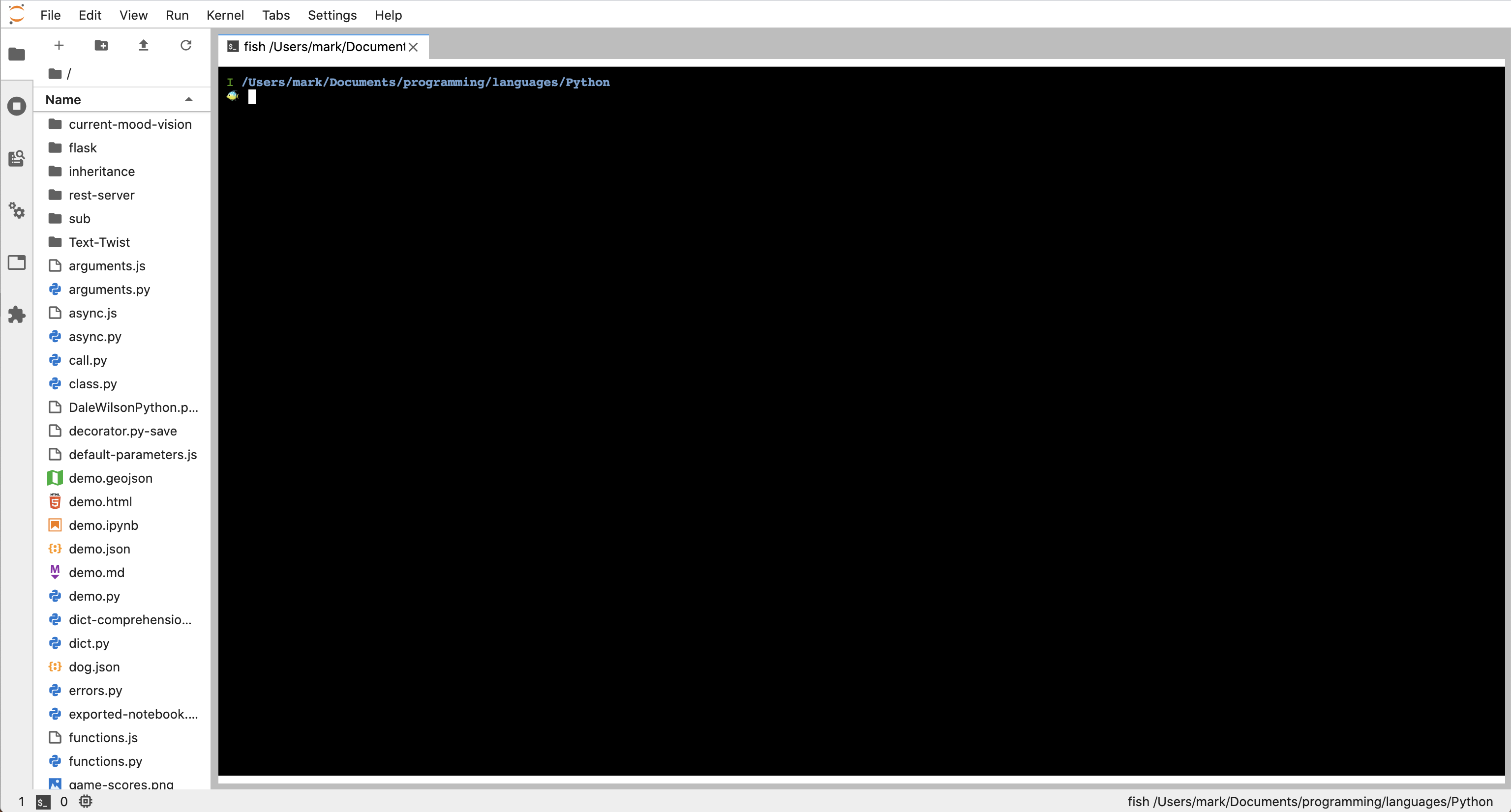
The terminal above uses the Fish Shell and the theme has been changed to “Dark”.
To change the terminal theme, select Settings … Terminal Theme … {theme} where the options are Inherit, Light, and Dark.
Tabs can be dragged to a new location similar to VS Code. This includes dragging them to new panes so the content of multiple tabs is visible at the same time.
Many image formats are supported and files that use them can be opened in a tab. Scroll to position the visible portion of the image. Press the ”=” and ”-” keys to zoom in and out. Press the ”[” and ”]” keys to rotate left and right. Press the “0” key to reset the zoom and rotation.
Other document formats that are supported include CSV, GeoJSON, HTML, JSON, Jupyter Notebooks, Latex, Markdown, PDF, and Vega.
CSV parsing is highly performant and a table view is lazily rendered, enabling processing of very large CSV files. The delimiter can be changed to comma, semicolon, tab, pipe, or hash.
Text Editor
To edit text files using preferred key bindings, select Settings … Text Editor Key Map … {key map name} where the options are default, Sublime Text, vim, and emacs. There are also extensions that enable use of Vim key bindings in notebook cells, but I haven’t been able to install one without errors.
To change the editor color theme, select Settings …Text Editor Theme … {theme name}. At last check there were 15 themes that include “solarized dark” and “solarized light”.
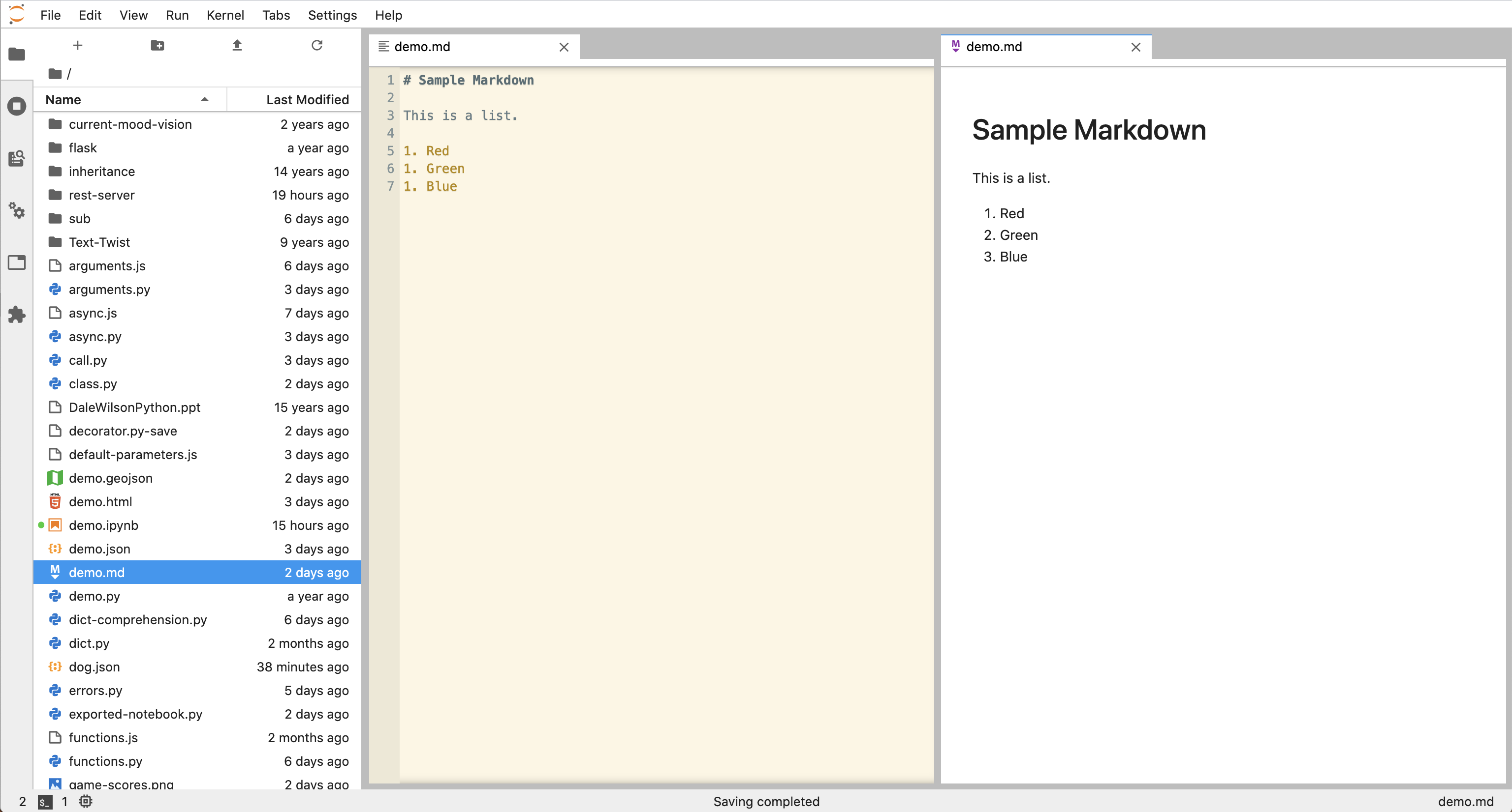
When editing Markdown files, to see a preview right-click and select “Show Markdown Preview”. This opens a new tab for the preview to the right of the tab containing Markdown text.
Jupyter Notebooks
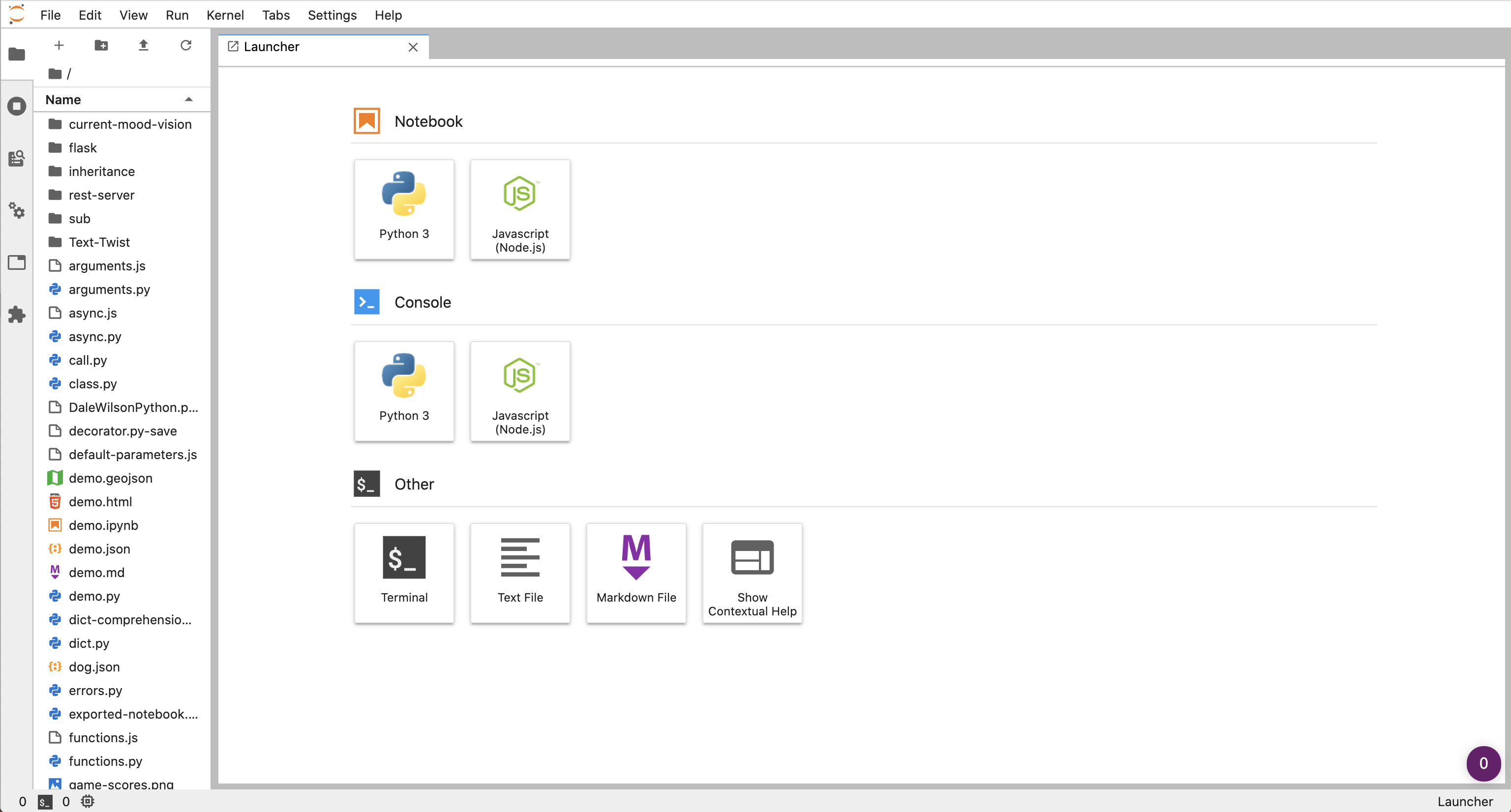
To create a new notebook, display the file browser in the left sidebar, click ”+” in the upper left to open a Launcher tab, and click the “Python 3” in the Notebook category. Alternatively, display the command palette in the left sidebar, type or select “New Notebook”, select the “Python 3” kernel in a dialog, and press the “Select” button. By default the only available kernel options are “Python 3” and “No Kernel”, but a JavaScript kernel and others can be added.
The new notebook will have the name “Untitled” followed by a number and the file extension “.ipynb” for “Interactive Python Notebook”. Notebooks are stored in JSON format. Their “cells” property is an array of objects that describe each cell.
To rename a notebook, right-click its tab and select “Rename Notebook”.
To open an existing notebook, double-click it in the file browser.
Notebooks open in command mode which supports navigating and changing the order of the cells. Press the up and down arrow keys to navigate between cells. The current cell is highlighted with a vertical blue bar.
Keyboard shortcuts
Keyboard shortcuts, many of which are borrowed from Vim, include:
| Action | Keyboard Shortcut |
|---|---|
| edit current cell | return |
| stop editing current cell, execute it, and advance to the next cell | shift-return |
| stop editing current cell, execute it, and remain on the current cell | ctrl-return |
| stop editing current cell and do not execute it | esc |
| add a cell above current one | a |
| add a cell below current one | b |
| copy current cell | c or press copy icon |
| delete current cell | dd or press scissors icon |
| move down one cell | j or down arrow |
| select current cell and next one down | shift-j or shift down arrow |
| move up one cell | k or up arrow |
| select current cell and previous one up | shift-k or shift up arrow |
| change format of current cell to Markdown | m |
| paste copied cell into current cell | v or press paste icon (clipboard) |
| cut current cell | x |
| change format of current cell to code | y |
| undo last action | z |
| redo last undo | shift-z |
| split current cell into two at cursor location | ctrl-shift-minus |
| see popup help for function after typing name | shift-tab |
Another way to select multiple cells starting from the current one is to shift-click the cell at the other end of the range, above or below the current one.
The current cell is indicated by a vertical blue bar to its left. Code cells also have a vertical blue bar to the left of their output. To collapse a cell or the output of a code cell, click the vertical blue bar. To expand, click the blue vertical line again. The View menu contains many menu items that collapse and expand sets of cells and outputs.
To reorder cells drag them up or down by the square brackets to their left to a new location. Another option is to cut the current cell, move to the cell it should be placed after, and paste it.
Yet another option is to customize key bindings. For example, ctrl-up arrow and ctrl-down arrow can be mapped to the “notebook:move-cell-up” and “notebook:move-cell-down” commands. To do this, select Settings … Advanced Settings Editor, select “Keyboard Shortcuts”, and add the following User Preferences:
{
  "shortcuts": [
    {
      "command": "notebook:move-cell-down",
      "keys": ["Ctrl ArrowDown"],
      "selector": "body"
    },
    {
      "command": "notebook:move-cell-up",
      "keys": ["Ctrl ArrowUp"],
      "selector": "body"
    }
  ]
}
To save changes in a file or notebook, click the floppy disk icon or press ctrl-s (cmd-s on Mac).
To view a notebook in multiple tabs, each of which can be scrolled to a different position, select File … New View for Notebook. Cells can be dragged from one view to another and even between notebooks. This copies the cell. There is not currently a way to move cells, but the original cell can be deleted after it has been copied to its new location.
To export a notebook containing Python code cells to a .py file,
select File … Export Notebook As … Export Notebook to Executable Script.
Select a directory, enter a file name, and press “Save”.
Markdown cells will appear as Python comments.
Code cells will be preceded by a comment that reads ”# In[{number}]”.
To export a notebook as a PDF file,
select File … Export Notebook As … Export Notebook to PDF.
This requires nbconvert and Pandoc be installed.
To install nbconvert, enter pip install nbconvert.
To install Pandoc in macOS, enter brew install pandoc xelatex.
Also see Install TeX for platform-specific install instructions.
This is a very large install! I did not try this.
Markdown Cells
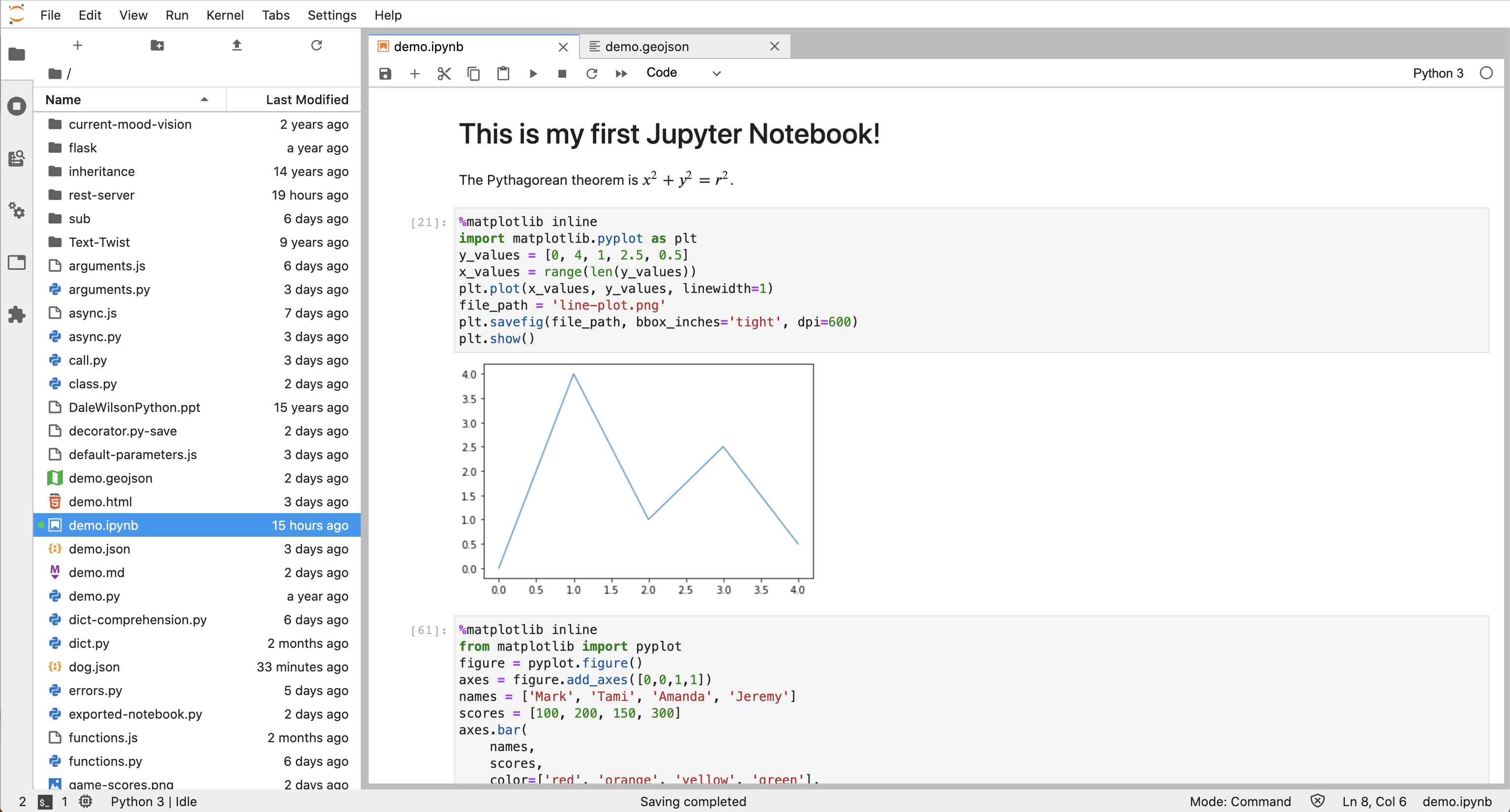
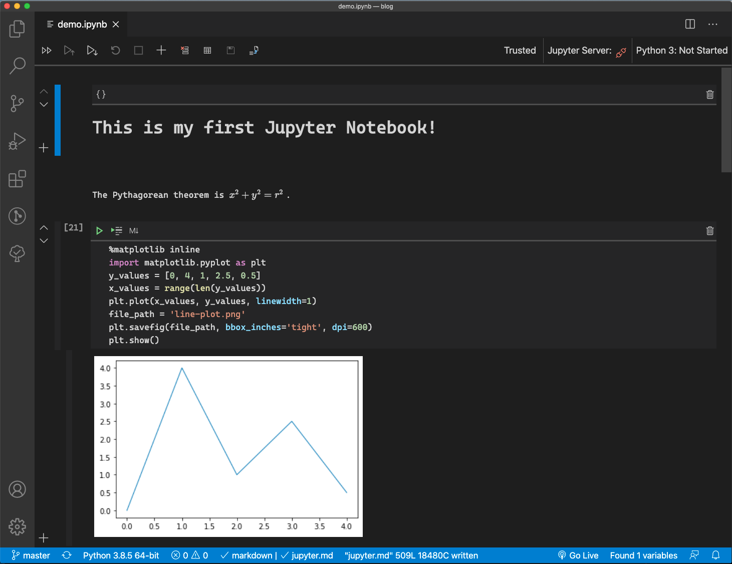
Markdown cells can contain equations surrounded by $ characters that will be nicely rendered. For example, “The Pythagorean theorem is $ x^2 + y^2 = r^2 $.” The previous screenshot shows how this is rendered.
URLs in Markdown cells are automatically converted to hyperlinks.
Code Cells
Code cells are automatically executed after leaving edit mode. Their output is displayed below the cell. If no output appears, look for error messages in the terminal where the Jupyter server is running.
To toggle the display of line numbers inside cells, select View … Show Line Numbers. Typically the number of lines in each cell is small enough that line numbers are not helpful.
The number in square brackets to the left of a cell indicates to the order in which the cell was executed relative to the other code cells. The number will be preceded by an asterisk while the code is running. This will only be visible for long running code. While it is running, the kernel is locked and no other cells can run. To stop execution of a long-running cell, generate a KeyboardInterrupt by clicking the black square at the top or pressing the “i” key twice. To demonstrate this, enter the following code in a cell and execute it:
from time import sleep
for i in range(10):
    print(i)
    sleep(1) # sleeps for one second
To execute a cell again without going into edit mode, select the cell and click the triangle at the top of the notebook. To re-execute all code cells, click the command palette icon in the left sidebar and enter or select “Run All Cells”.
Variables defined in preceding code cells are available in cells that follow.
Ending a cell with a variable name causes its value to be output
without using a print statement.
A code cell can import and use locally-defined modules.
For example, the following works if the file statistics.py exists
and defines a class named Statistics that has a report method:
from statistics import Statistics
stats = Statistics(1, 2, 3, 4, 5, 6)
stats.report()
For more tips, see Jupyter Notebook Tips, Tricks, & Shortcuts.
JavaScript Kernel
Jupyter supports Python out of the box. Additional language kernels can be installed to support other programming languages. These implement the Jupyter messaging protocol.
IJavascript is a Jupyter kernel for JavaScript. To install it:
- Install Node.js.
- See the installation at
IJavaScript Installation.
On macOS:
brew install pkg-config zeromqsudo easy_install pippip install --upgrade pyzmq jupyternpm install -g ijavascriptijsinstall
To create a “Javascript (Node.js)” notebook, click the File Explorer icon in the left sidebar, click the ”+” at the top of the left sidebar, and click the “JS” box under the “Notebook” section. Cells that have a type of “Code” can contain and execute JavaScript code.
Plots
There are many libraries that can be used to create plots inside Jupyter.
A popular option is matplotlib.
To install it, enter pip install matplotlib.
To draw a line chart, save it to a PNG file, and display it, enter the following in a cell and execute it:
%matplotlib inline
import matplotlib.pyplot as plt
y_values = [0, 4, 1, 2, 0.5]
x_values = range(len(y_values))
plt.plot(x_values, y_values, linewidth=1)
# Save plot as a PNG file.
plt.savefig('line-plot.png', bbox_inches='tight', dpi=600)
plt.show()

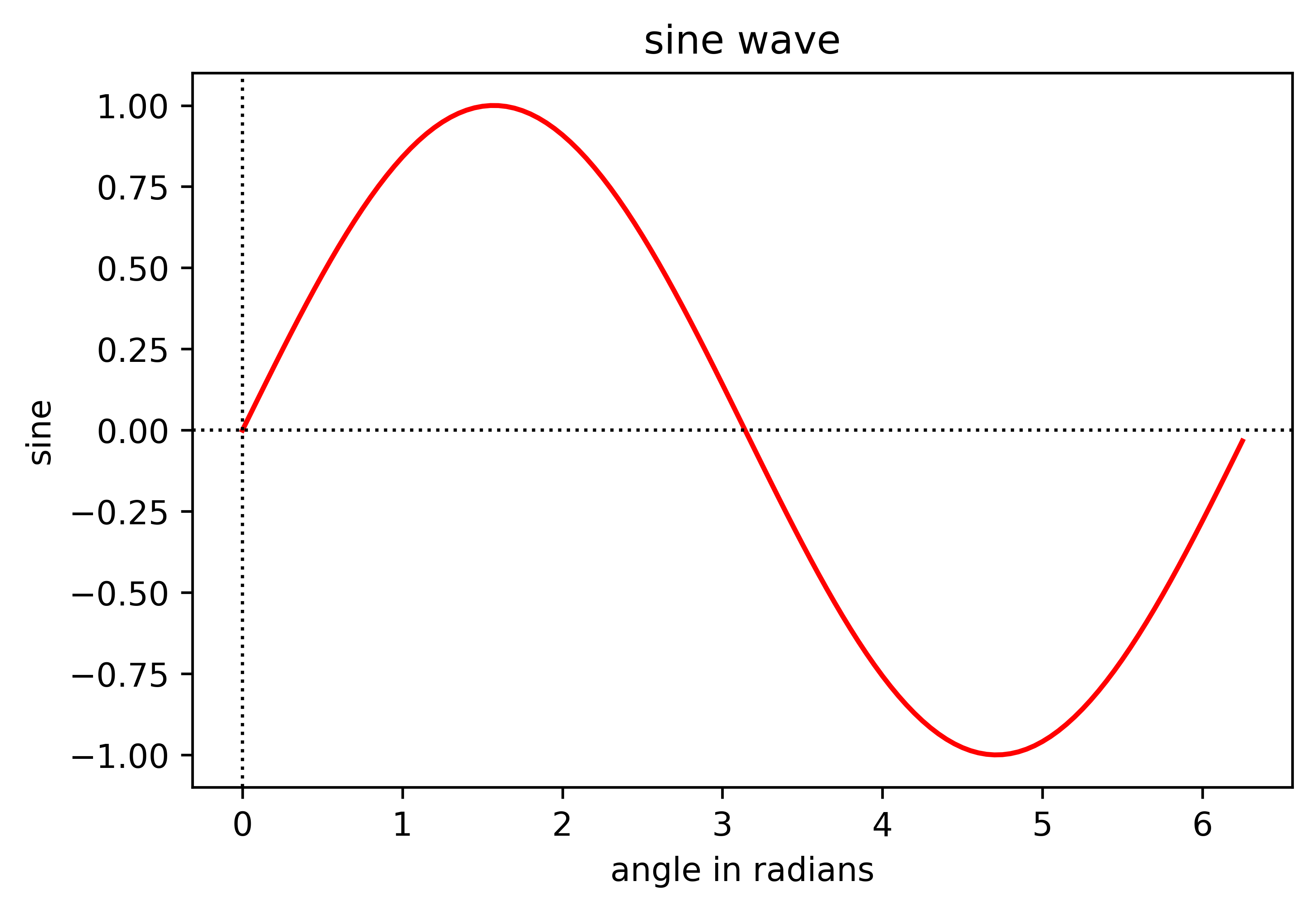
To plot a function, enter the following in a cell and execute it:
from matplotlib import pyplot as plt
import numpy as np
import math # for pi
step_size = 0.05
min_x = 0
#min_x = -5 #0
max_x = math.pi * 2
#max_x = 5
x = np.arange(min_x, max_x, step_size)
y = np.sin(x)
#y = x**2
plt.plot(x, y, color='red')
plt.axhline(0, color='black', linestyle="dotted", linewidth=1) # x axis
plt.axvline(0, color='black', linestyle="dotted", linewidth=1) # y axis
plt.xlabel('angle in radians')
plt.ylabel('sine')
plt.title('sine wave')
plt.savefig('sine-wave.png', bbox_inches='tight', dpi=600)
plt.show()
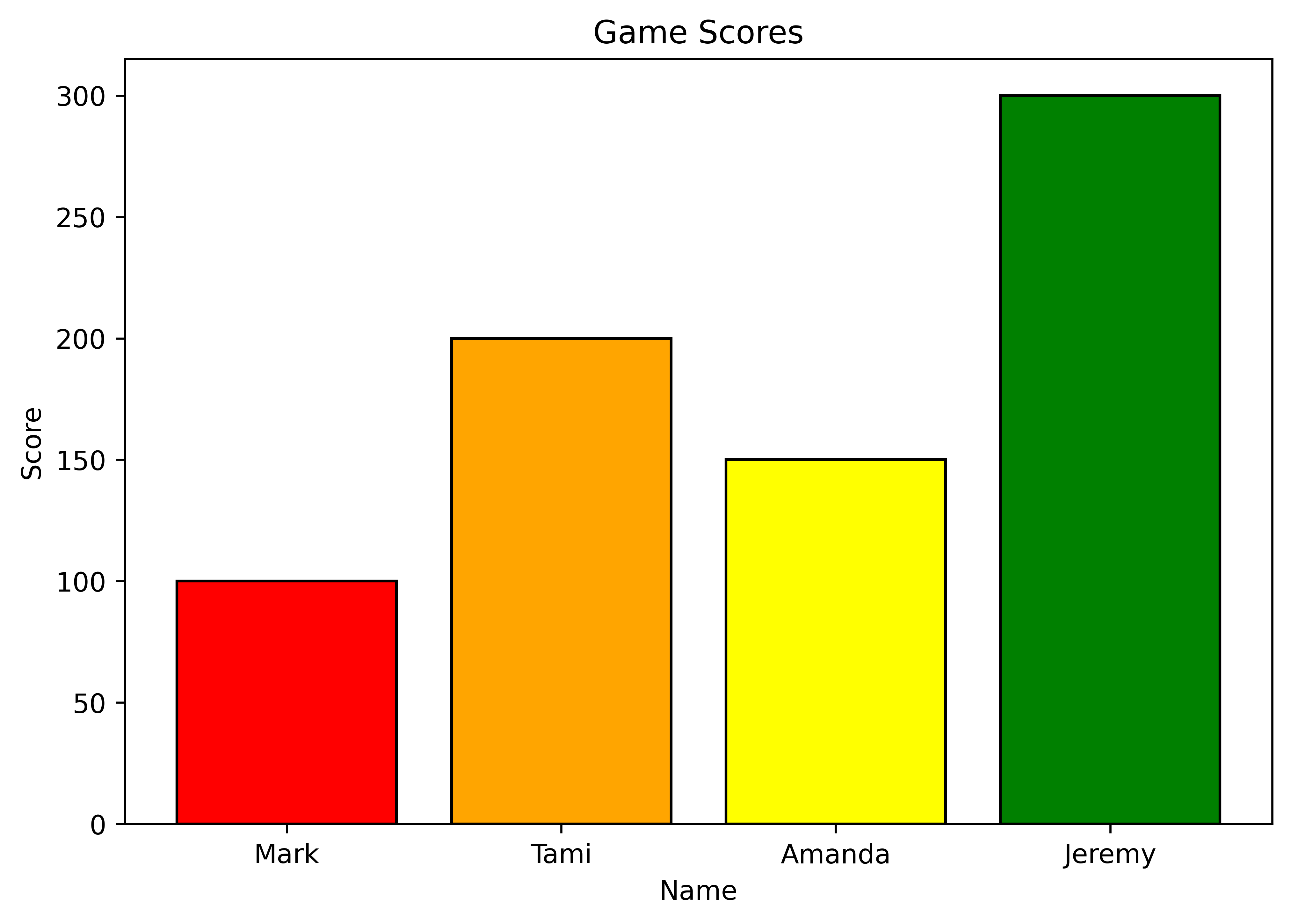
To draw a bar chart, enter the following in a cell and execute it:
%matplotlib inline
from matplotlib import pyplot as plt
figure = plt.figure()
axes = figure.add_axes([0,0,1,1])
names = ['Mark', 'Tami', 'Amanda', 'Jeremy']
scores = [100, 200, 150, 300]
axes.bar(
    names,
    scores,
    color=['red', 'orange', 'yellow', 'green'],
    edgecolor='black')
axes.set_title('Game Scores')
axes.set_xlabel('Name')
axes.set_ylabel('Score')
plt.savefig('game-scores.png', bbox_inches='tight', dpi=600)
plt.show()
Vega
Vega
is a JSON format for describing data visualizations.
Jupyter has built-in support for rendering Vega files
with a .vg or .vg.json file extension.
There are many examples at the Vega website linked above.
Copy the JSON for one into a .vg file
and open it in Jupyter to see the result.
An example of a Vega line chart can be found at Line Chart Example. It produces the following chart:

Click the circled ellipsis in the upper-right corner of the chart (not shown above) to display a menu where you can select “Save as SVG”, “Save as PNG”, “View Source” (displays read-only text in a new browser tab), or “Open in Vega Editor” (opens Vega online editor in a new browser tab). Changes made in the Vega editor can be exported as JSON and reopened in Jupyter.
GeoJSON
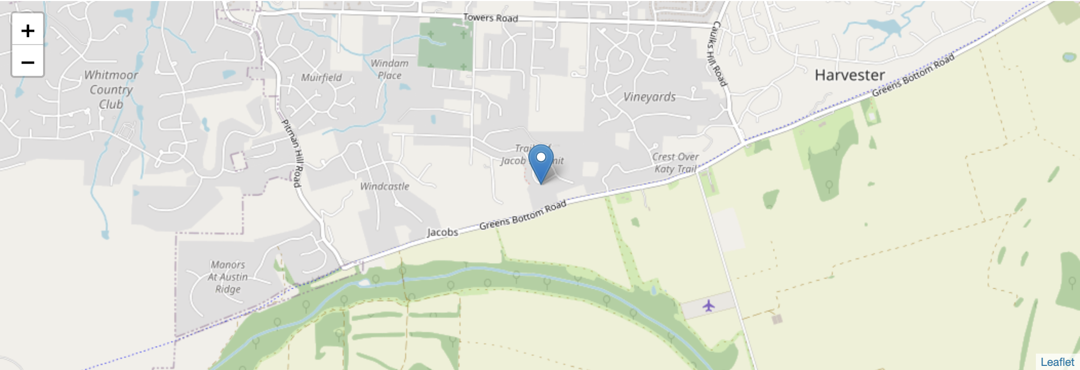
To render GeoJSON data in Jupyter:
- Install an extension by entering
jupyter labextension install @jupyterlab/geojson-extension - You may need to restart the Jupyter server.
- Enter code like the following in a cell of a Python notebook:
from IPython.display import GeoJSON
data = {
    'type': 'Feature',
    'geometry': {
        'type': 'Point',
        'coordinates': [-118.4563712, 34.0163116]
        #'coordinates': [-90.594482, 38.709419]
    }
}
# minZoom defaults to 0 and maxZoom defaults to 18.
# When minZoom is 0 or 1, parts of the world are visible more than once,
# so setting it to 2 or above is recommended.
# When maxZoom is >= 20, no map is rendered,
# so setting it to 19 or below is recommended.
# The map starts at maxZoom.
GeoJSON(data, layer_options={'minZoom': 2, 'maxZoom': 19})
VS Code
VS Code supports creating, rendering, and editing Jupyter Notebooks. To enable this, open the Command Palette and select “Python: Select Python Interpreter to start Jupyter server” and select an installed Python interpreter.
To create a new notebook, open the Command Palette and select “Python: Create Blank New Jupyter Notebook”.
Opening an existing .ipynb notebook file renders it in a new VS Code tab.
When rendering data visualizations,
VS Code will ask if ipykernel should be installed.
Press the “Yes” button.
The user interface is slightly different than the JupyterLab web UI.
- Cells and their output cannot be collapsed.
- To add a new cell after an existing one, click the ”+” to its left. The ”+” at the top of the window can be clicked to add a new cell after the currently selected cell.
- To delete a cell, click the trash can icon in its upper-right.
- Cells cannot be dragged to a new location. Instead the up and down angles to the left of each cell can be clicked to move the cell up or down.
- To run the code in a cell, click the green triangle at the top of the cell.
- To step through the code in a cell, executing one line at a time, repeatedly click the icon containing a small green triangle at the top of the cell.
- To stop a long running cell, click the red square at the top of the cell or the one at the top of the window.
- To clear the output of all cells, click the icon with three cells and a small red “x” at the top of the window.
- To run the code in all cells, click the double triangle icon at the top of the window.
Methods in matplotlab that save plots to files do not seem to work when called inside VS Code.
For more details, see Working with Jupyter Notebooks in Visual Studio Code.
Resources
For help, join the Jupyter Discourse by browsing the Community page and clicking the “View” button for “Jupyter Discourse”.